R (programming language)
 R terminal | |
| Paradigms | Multi-paradigm: procedural, object-oriented, functional, reflective, imperative, array[1] |
|---|---|
| Designed by | Ross Ihaka and Robert Gentleman |
| Developer | R Core Team |
| First appeared | August 1993 |
| Typing discipline | Dynamic |
| Platform | arm64 and x86-64 |
| License | GNU GPL v2[2] |
| Filename extensions | |
| Website | {{{1}}} |
| Influenced by | |
| Influenced | |
| Julia[6] | |
| |
R is a programming language for statistical computing and data visualization. Created by statisticians Ross Ihaka and Robert Gentleman, R has been adopted in the fields of data mining, bioinformatics, and data analysis.[7]
The core R language is augmented by a large number of extension packages, containing reusable code, documentation, and sample data.
R software is open-source free software, licensed by the GNU Project, and available under the GNU General Public License.[2] It is written primarily in C, Fortran, and R itself. Precompiled executables are provided for various operating systems. R is supported by the R Core Team[8] and the R Foundation for Statistical Computing.[9]
R has a native command line interface. Moreover, multiple third-party graphical user interfaces are available, such as RStudio—an integrated development environment—and Jupyter—a notebook interface.
History
.jpg)
R was started by professors Ross Ihaka and Robert Gentleman as a programming language to teach introductory statistics at the University of Auckland.[10] The language was inspired by the S programming language, with most S programs able to run unaltered in R.[5] The language was also inspired by Scheme's lexical scoping, allowing for local variables.[1]
The name of the language, R, comes from being both an S language successor as well as the shared first letter of the authors, Ross and Robert.[11] In August 1993, Ihaka and Gentleman posted a binary of R on the data archive StatLib and announced the posting on the s-news mailing list.[12] On April 1, 1997, the mailing list for the R Project began, preceding the release of version 0.50.[13] On December 5, 1997, R became a GNU project when version 0.60 was released.[14] On February 29, 2000, the first official 1.0 version was released.[15]
The Comprehensive R Archive Network (CRAN) was founded in 1997 by Kurt Hornik and Fritz Leisch to host R's source code, executable files, documentation, and user-created packages.[16] Its name and scope mimic the Comprehensive TeX Archive Network and the Comprehensive Perl Archive Network.[16] CRAN originally had three mirrors and 12 contributed packages.[17] As of December 2022, it has 103 mirrors[18] and 18,976 contributed packages.[19]
The R Core Team was formed in 1997 to further develop the language.[20] In April 2003, the R Foundation was founded as a non-profit organization to provide further support for the R Project.[20]
Examples
Mean -- a measure of center
A numeric data set may have a central tendency — where some of the most typical data points reside.[21] The arithmetic mean (average) is the most commonly used measure of central tendency.[21] The mean of a numeric data set is the sum of the data points divided by the number of data points.[21]
- Let [math]\displaystyle{ \bar{x} }[/math] = the mean of a data set.
- Let [math]\displaystyle{ x }[/math] = a list of data points.
- Let [math]\displaystyle{ n }[/math] = the number of data points.
- [math]\displaystyle{ \bar{x} = \frac{x_1+x_2+\cdots +x_n}{n} }[/math]
Suppose a sample of four observations of Celsius temperature measurements were taken 12 hours apart.
- Let [math]\displaystyle{ x }[/math] = a list of degrees Celsius data points of 30, 27, 31, 28.
This R computer program will output the mean of [math]\displaystyle{ x }[/math]:
# The c() function "combines" a list into a single object.
x <- c( 30, 27, 31, 28 )

sum <- sum( x )
length <- length( x )
mean <- sum / length

message( "Mean:" )
print( mean )
Note: R can have the same identifier represent both a function name and its result. For more information, visit scope.
Output:
Mean:
[1] 29
This R program will execute the native mean() function to output the mean of [math]\displaystyle{ }[/math]x:
x <- c( 30, 27, 31, 28 )

message( "Mean:" )
print( mean( x ) )
Output:
Mean:
[1] 29
Standard Deviation -- a measure of dispersion
A standard deviation of a numeric data set is an indication of the average distance all the data points are from the mean.[22] For a data set with a small amount of variation, then each data point will be close to the mean, so the standard deviation will be small.[22]
- Let [math]\displaystyle{ s }[/math] = the standard deviation of a data set.
- Let [math]\displaystyle{ x }[/math] = a list of data points.
- Let [math]\displaystyle{ n }[/math] = the number of data points.
- [math]\displaystyle{ s = \sqrt{\frac{\sum\left(x_i - \bar{x}\right)^2}{n - 1}} }[/math]
Suppose a sample of four observations of Celsius temperature measurements were taken 12 hours apart.
- Let [math]\displaystyle{ x }[/math] = a list of degrees Celsius data points of 30, 27, 31, 28.
This R program will output the standard deviation of [math]\displaystyle{ x }[/math]:
x <- c( 30, 27, 31, 28 )
distanceFromMean <- x - mean( x )
distanceFromMeanSquared <- distanceFromMean ** 2
distanceFromMeanSquaredSum <- sum( distanceFromMeanSquared )
variance <- distanceFromMeanSquaredSum / ( length( x ) - 1 )
standardDeviation <- sqrt( variance )

message( "Standard Deviation:" )
print( standardDeviation )
Output:
Standard Deviation:
[1] 1.825742
This R program will execute the native sd() function to output the standard deviation of [math]\displaystyle{ x }[/math]:
x <- c( 30, 27, 31, 28 )

message( "Standard Deviation:" )
print( sd( x ) )
Output:
Standard Deviation:
[1] 1.825742
Linear regression -- a measure of relation

A phenomenon may be the result of one or more observable events. For example, the phenomenon of skiing accidents may be the result of having snow in the mountains. A method to measure whether or not a numeric data set is related to another data set is linear regression.[24]
- Let [math]\displaystyle{ x }[/math] = a data set of independent data points, in which each point occurred at a specific time.
- Let [math]\displaystyle{ y }[/math] = a data set of dependent data points, in which each point occurred at the same time of an independent data point.
If a linear relationship exists, then a scatter plot of the two data sets will show a pattern that resembles a straight line.[25] If a straight line is embedded into the scatter plot such that the average distance from all the points to the line is minimal, then the line is called a regression line. The equation of the regression line is called the regression equation.[26]
The regression equation is a linear equation; therefore, it has a slope and y-intercept. The format of the regression equation is [math]\displaystyle{ \hat{y} = b_{0} + b_{1}x }[/math].[27][lower-alpha 1]
- Let [math]\displaystyle{ b_{1} }[/math] = the slope of the regression equation.
- [math]\displaystyle{ b_{1} = \frac{\sum\left(x - \bar{x}\right)\left(y - \bar{y}\right)}{\sum\left(x - \bar{x}\right)^2} }[/math]
- Let [math]\displaystyle{ b_{0} }[/math] = the y-intercept of the regression equation.
- [math]\displaystyle{ b_{0} = \bar{y} - b_{1}\bar{x} }[/math]
Suppose a sample of four observations of Celsius temperature measurements were taken 12 hours apart. At the same time, the thermometer was switched to Fahrenheit temperature and another measurement was taken.
- Let [math]\displaystyle{ x }[/math] = a list of degrees Celsius data points of 30, 27, 31, 28.
- Let [math]\displaystyle{ y }[/math] = a list of degrees Fahrenheit data points of 86.0, 80.6, 87.8, 82.4.
This R program will output the slope and y-intercept of a linear relationship in which [math]\displaystyle{ y }[/math] depends upon [math]\displaystyle{ x }[/math]:
x <- c( 30, 27, 31, 28 )
y <- c( 86.0, 80.6, 87.8, 82.4 )

# Build the numerator
independentDistanceFromMean <- x - mean( x )
sampledDependentDistanceFromMean <- y - mean( y )

independentDistanceTimesSampledDistance <-
    independentDistanceFromMean *
    sampledDependentDistanceFromMean

independentDistanceTimesSampledDistanceSum <-
    sum( independentDistanceTimesSampledDistance )

# Build the denominator
independentDistanceFromMeanSquared <-
    independentDistanceFromMean ** 2

independentDistanceFromMeanSquaredSum <-
    sum( independentDistanceFromMeanSquared )

# Slope is rise over run
slope <-
    independentDistanceTimesSampledDistanceSum /
    independentDistanceFromMeanSquaredSum

yIntercept <- mean( y ) - slope * ( mean( x ) )

message( "Slope:" )
print( slope )

message( "Y-intercept:" )
print( yIntercept )
Output:
Slope:
[1] 1.8
Y-intercept:
[1] 32
This R program will execute the native functions to output the slope and y-intercept:
x <- c( 30, 27, 31, 28 )
y <- c( 86.0, 80.6, 87.8, 82.4 )

# Execute lm() with Fahrenheit depends upon Celsius
linearModel <- lm( y ~ x )

# coefficients() returns a structure containing the slope and y intercept
coefficients <- coefficients( linearModel )

# Extract the slope from the structure
slope <- coefficients"x"

# Extract the y intercept from the structure
yIntercept <- coefficients"(Intercept)"

message( "Slope:" )
print( slope )

message( "Y-intercept:" )
print( yIntercept )
Output:
Slope:
[1] 1.8
Y-intercept:
[1] 32
The coefficient of determination determines the percentage of variation explained by the independent variable.[28] It always lies between 0 and 1.[29] A value of 0 indicates no relationship between the two data sets, and a value near 1 indicates the regression equation is extremely useful for making predictions.[30]
- Let [math]\displaystyle{ \hat{y} }[/math] = the data set of predicted response data points when the independent data points are passed through the regression equation.
- Let [math]\displaystyle{ r^{2} }[/math] = the coefficient of determination in a relationship between an independent variable and a dependent variable.
- [math]\displaystyle{ r^{2} = \frac{\sum\left(\hat{y} - \bar{y}\right)^2}{\sum\left(y - \bar{y}\right)^2} }[/math]
This R program will output the coefficient of determination of the linear relationship between [math]\displaystyle{ x }[/math] and [math]\displaystyle{ y }[/math]:
x <- c( 30, 27, 31, 28 )
y <- c( 86.0, 80.6, 87.8, 82.4 )

# Build the numerator
linearModel <- lm( y ~ x )
coefficients <- coefficients( linearModel )
slope <- coefficients"x"
yIntercept <- coefficients"(Intercept)"
predictedResponse <- yIntercept + ( slope * x )

predictedResponseDistanceFromMean <-
    predictedResponse - mean( y )

predictedResponseDistanceFromMeanSquared <-
    predictedResponseDistanceFromMean ** 2

predictedResponseDistanceFromMeanSquaredSum <-
    sum( predictedResponseDistanceFromMeanSquared )

# Build the denominator
sampledResponseDistanceFromMean <- y - mean( y )

sampledResponseDistanceFromMeanSquared <-
    sampledResponseDistanceFromMean ** 2

sampledResponseDistanceFromMeanSquaredSum <-
    sum( sampledResponseDistanceFromMeanSquared )

coefficientOfDetermination <-
    predictedResponseDistanceFromMeanSquaredSum /
    sampledResponseDistanceFromMeanSquaredSum

message( "Coefficient of Determination:" )
print( coefficientOfDetermination )
Output:
Coefficient of Determination:
[1] 1
This R program will execute the native functions to output the coefficient of determination:
x <- c( 30, 27, 31, 28 )
y <- c( 86.0, 80.6, 87.8, 82.4 )

linearModel <- lm( y ~ x )
summary <- summary( linearModel )
coefficientOfDetermination <- summary"r.squared"

message( "Coefficient of Determination:" )
print( coefficientOfDetermination )
Output:[lower-alpha 2]
Coefficient of Determination:
[1] 1
Single plot
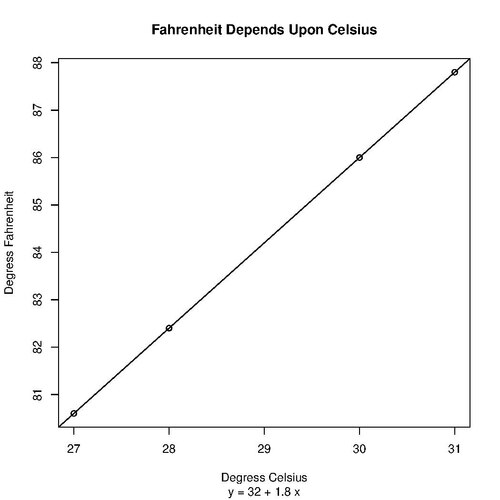
This R program will display a scatter plot with an embedded regression line and regression equation illustrating the relationship between [math]\displaystyle{ x }[/math] and [math]\displaystyle{ y }[/math]:
x <- c( 30, 27, 31, 28 )
y <- c( 86.0, 80.6, 87.8, 82.4 )

linearModel <- lm( y ~ x )
coefficients <- coefficients( linearModel )
slope <- coefficients"x"
intercept <- coefficients"(Intercept)"

# Execute paste() to build the regression equation string
regressionEquation <- paste( "y =", intercept, "+", slope, "x" )

# Display a scatter plot with the regression line and equation embedded
plot(
    x,
	y,
	main = "Fahrenheit Depends Upon Celsius",
	sub = regressionEquation,
	xlab = "Degress Celsius",
	ylab = "Degress Fahrenheit",
	abline( linearModel ) )
Output:
Multi plot
This R program will generate a multi-plot and a table of residuals.
# The independent variable is a list of numbers 1 to 6.
x <- 1:6

# The dependent variable is a list of each independent variable squared.
y <- x^2

# Executing the linear model on a quadratic equation will produce residuals.
linearModel <- lm(y ~ x)

# Display the residuals.
summary( linearModel )

# Create a 2 by 2 multi-plot.
par(mfrow = c(2, 2))

# Output the multi-plot.
plot( linearModel )
Output:
Residuals:
      1       2       3       4       5       6       7       8      9      10
 3.3333 -0.6667 -2.6667 -2.6667 -0.6667  3.3333

Coefficients:
            Estimate Std. Error t value Pr(>|t|)
(Intercept)  -9.3333     2.8441  -3.282 0.030453 *
x             7.0000     0.7303   9.585 0.000662 ***
---
Signif. codes:  0 ‘***’ 0.001 ‘**’ 0.01 ‘*’ 0.05 ‘.’ 0.1 ‘ ’ 1

Residual standard error: 3.055 on 4 degrees of freedom
Multiple R-squared:  0.9583, Adjusted R-squared:  0.9478
F-statistic: 91.88 on 1 and 4 DF,  p-value: 0.000662

Mandelbrot graphic
This Mandelbrot set example highlights the use of complex numbers. It models the first 20 iterations of the equation z = z2 + c, where c represents different complex constants.
Install the package that provides the write.gif() function beforehand:
install.packages("caTools")
R program:
library(caTools)

jet.colors <-
    colorRampPalette(
        c("green", "pink", "#007FFF", "cyan", "#7FFF7F",
          "white", "#FF7F00", "red", "#7F0000"))

dx <- 1500 # define width
dy <- 1400 # define height

C  <-
    complex(
        real =
            rep(
                seq(-2.2, 1.0, length.out = dx), each = dy),
                imag = rep(seq(-1.2, 1.2, length.out = dy),
                dx))

# reshape as matrix of complex numbers
C <- matrix(C, dy, dx)

# initialize output 3D array
X <- array(0, c(dy, dx, 20))

Z <- 0

# loop with 20 iterations
for (k in 1:20) {

  # the central difference equation
  Z <- Z^2 + C

  # capture the results
  X[, , k] <- exp(-abs(Z))
}

write.gif(
    X,
    "Mandelbrot.gif",
    col = jet.colors,
    delay = 100)
Output:

Programming
R is an interpreted language, so programmers typically access it through a command-line interpreter. If a programmer types 1+1 at the R command prompt and presses enter, the computer replies with 2.[31] Programmers also save R programs to a file then execute the batch interpreter Rscript.[32]
Object
R stores data inside an object. An object is assigned a name which the computer program uses to set and retrieve the data.[33] An object is created by placing its name to the left of the symbol pair <-.[34]
To create an object named x and assign it the integer 82:
x <- 82L
print( x )
Output:
[1] 82
The [1] displayed before the number is a subscript. It shows the container for this integer is index one of an array.
Vector
The most primitive R object is the vector.[35] A vector is a one dimensional array of data. To assign multiple elements to the array, use the c() function to "combine" the elements. The elements must be the same data type.[36] R lacks scalar data types, which are placeholders for a single word — usually an integer. Instead, a single integer is stored into the first element of an array. The single integer is retrieved using the index subscript of [1].[lower-alpha 3]
R program to store and retrieve a single integer:
store <- 82L
retrieve <- store[1]
print( retrieve[1] )
Output:
[1] 82
Element-wise operation
When an operation is applied to a vector, R will apply the operation to each element in the array. This is called an element-wise operation.[37]
This example creates the object named x and assigns it integers 1 through 3. The object is displayed and then again with one added to each element:
x <- 1:3
print( x )
print( x + 1 )
Output:
[1] 1 2 3
[1] 2 3 4
To achieve the many additions, R implements vector recycling.[37] The number one following the + operation is converted into an internal array of three ones. The + operation simultaneously loops through both arrays and performs the addition on each element pair. The results are stored into another internal array of three elements which is returned to the print() function.
Numeric vector
A numeric vector is used to store integers and floating point numbers.[38] The primary characteristic of a numeric vector is the ability to perform arithmetic on the elements.[38]
Integer vector
By default, integers (numbers without a decimal point) are stored as floating point. To force integer memory allocation, append an L to the number. As an exception, the sequence operator : will, by default, allocate integer memory.
R program:
x <- 82L
print( x[1] )
message( "Data type:" )
typeof( x )
Output:
[1] 82
Data type:
[1] "integer"
R program:
x <- c( 1L, 2L, 3L )
print( x )
message( "Data type:" )
typeof( x )
Output:
[1] 1 2 3
Data type:
[1] "integer"
R program:
x <- 1:3
print( x )
message( "Data type:" )
typeof( x )
Output:
[1] 1 2 3
Data type:
[1] "integer"
Double vector
A double vector stores real numbers, which are also known as floating point numbers. The memory allocation for a floating point number is double precision.[38] Double precision is the default memory allocation for numbers with or without a decimal point.
R program:
x <- 82
print( x[1] )
message( "Data type:" )
typeof( x )
Output:
[1] 82
Data type:
[1] "double"
R program:
x <- c( 1, 2, 3 )
print( x )
message( "Data type:" )
typeof( x )
Output:
[1] 1 2 3
Data type:
[1] "double"
Logical vector
A logical vector stores binary data — either TRUE or FALSE. The purpose of this vector is to store the result of a comparison.[39] A logical datum is expressed as either TRUE, T, FALSE, or F.[39] The capital letters are required, and no quotes surround the constants.[39]
R program:
x <- 3 < 4
print( x[1] )
message( "Data type:" )
typeof( x )
Output:
[1] TRUE
Data type:
[1] "logical"
Two vectors may be compared using the following logical operators:[40]
| Operator | Syntax | Tests |
|---|---|---|
| > | a > b | Is a greater than b? |
| >= | a >= b | Is a greater than or equal to b? |
| < | a < b | Is a less than b? |
| <= | a <= b | Is a less than or equal to b? |
| == | a == b | Is a equal to b? |
| != | a != b | Is a not equal to b? |
Character vector
A character vector stores character strings.[41] Strings are created by surrounding text in double quotation marks.[41]
R program:
x <- "hello world"
print( x[1] )
message( "Data type:" )
typeof( x )
Output:
[1] "hello world"
Data type:
[1] "character"
R program:
x <- c( "hello", "world" )
print( x )
message( "Data type:" )
typeof( x )
Output:
[1] "hello" "world"
Data type:
[1] "character"
Factor
A Factor is a vector that stores a categorical variable.[42] The factor function converts a text string into an enumerated type, which is stored as an integer.[43]
In experimental design, a factor is an independent variable to test (an input) in a controlled experiment.[44] A controlled experiment is used to establish causation, not just association.[45] For example, one could notice that an increase in hot chocolate sales is associated with an increase in skiing accidents.
An experimental unit is an item that an experiment is being performed upon. If the experimental unit is a person, then it is known as a subject. A response variable (also known as a dependent variable) is a possible outcome from an experiment. A factor level is a characteristic of a factor. A treatment is an environment consisting of a combination of one level (characteristic) from each of the input factors. A replicate is the execution of a treatment on an experimental unit and yields response variables.[46]
This example builds two R programs to model an experiment to increase the growth of a species of Cactus. Two factors are tested:
- water levels of none, light, or medium
- superabsorbent polymer levels of not used or used
R program to setup the design:
# Step 1 is to establish the levels of a factor.
# Vector of the water levels:
waterLevel <-
    c(
        "none",
        "light",
        "medium" )

# Step 2 is to create the factor.
# Vector of the water factor:
waterFactor <-
    factor(
        # Although a subset is possible, use all of the levels.
        waterLevel,
        levels = waterLevel )

# Vector of the polymer levels:
polymerLevel <-
    c(
        "notUsed",
        "used" )

# Vector of the polymer factor:
polymerFactor <-
    factor(
        polymerLevel,
        levels = polymerLevel )

# The treatments are the cartesian product of both factors.
treatment_cartesian_product <-
    expand.grid(
        waterFactor,
        polymerFactor )

message( "Water factor:" )
print( waterFactor )

message( "\nPolymer factor:" )
print( polymerFactor )

message( "\nTreatment cartesian product:" )
print( treatment_cartesian_product )
Output:
Water factor:
[1] none   light  medium
Levels: none light medium

Polymer factor:
[1] notUsed used
Levels: notUsed used

Treatment cartesian product:
    Var1    Var2
1   none notUsed
2  light notUsed
3 medium notUsed
4   none    used
5  light    used
6 medium    used
R program to store and display the results:
experimentalUnit <- c( "plant1", "plant2", "plant3" )

replicateWater <- c( "none", "light", "medium" )
replicatePolymer <- c( "notUsed", "used", "notUsed" )
replicateInches <- c( 82L, 83L, 84L )

response <-
    data.frame(
        experimentalUnit,
        replicateWater,
        replicatePolymer,
        replicateInches )

print( response )
Output:
experimentalUnit replicateWater replicatePolymer replicateInches
1          plant1            none          notUsed              82
2          plant2           light             used              83
3          plant3          medium          notUsed              84
Data frame
A data frame stores a two-dimensional array.[47] The horizontal dimension is a list of vectors. The vertical dimension is a list of rows. It is the most useful structure for data analysis.[48] Data frames are created using the data.frame() function. The input is a list of vectors (of any data type). Each vector becomes a column in a table. The elements in each vector are aligned to form the rows in the table.
R program:
integer <- c( 82L, 83L )
string <- c( "hello", "world" )
data.frame <- data.frame( integer, string )
print( data.frame )
message( "Data type:" )
class( data.frame )
Output:
integer string
1      82  hello
2      83  world
Data type:
[1] "data.frame"
Data frames can be deconstructed by providing a vector's name between double brackets. This returns the original vector. Each element in the returned vector can be accessed by its index number.
R program to extract the word "world". It is stored in the second element of the "string" vector:
integer <- c( 82L, 83L )
string <- c( "hello", "world" )
data.frame <- data.frame( integer, string )
vector <- data.frame"string"
print( vector[2] )
message( "Data type:" )
typeof( vector )
Output:
[1] "world"
Data type:
[1] "character"
Vectorized coding
Vectorized coding is a method to produce quality R computer programs that take advantage of R's strengths.[49] The R language is designed to be fast at logical testing, subsetting, and element-wise execution.[49] On the other hand, R does not have a fast for loop.[50] For example, R can search-and-replace faster using logical vectors than by using a for loop.[50]
For loop
A for loop repeats a block of code for a specific amount of iterations.[51]
Example to search-and-replace using a for loop:
vector <- c( "one", "two", "three" )

for ( i in 1:length( vector ) )
{
    if ( vector[ i ] == "one" )
    {
        vector[ i ] <- "1"
    }
}

message( "Replaced vector:" )
print( vector )
Output:
Replaced vector:
[1] "1"  "two" "three"
Subsetting
R's syntax allows for a logical vector to be used as an index to a vector.[52] This method is called subsetting.[53]
R example:
vector <- c( "one", "two", "three" )

print( vector[ c( TRUE, FALSE, TRUE ) ] )
Output:
[1] "one" "three"
Change a value using an index number
R allows for the assignment operator <- to overwrite an existing value in a vector by using an index number.[54]
R example:
vector <- c( "one", "two", "three" )
vector[ 1 ] <- "1"

print( vector )
Output:
[1] "1" "two" "three"
Change a value using subsetting
R also allows for the assignment operator <- to overwrite an existing value in a vector by using a logical vector.
R example:
vector <- c( "one", "two", "three" )
vector[ c( TRUE, FALSE, FALSE ) ] <- "1"

print( vector )
Output:
[1] "1" "two" "three"
Vectorized code to search-and-replace
Because a logical vector may be used as an index, and because the logical operator returns a vector, a search-and-replace can take place without a for loop.
R example:
vector <- c( "one", "two", "three" )
vector[ vector == "one" ] <- "1"

print( vector )
Output:
[1] "1" "two" "three"
Functions
A function is an object that stores computer code instead of data.[55] The purpose of storing code inside a function is to be able to reuse it in another context.[55]
Native functions
R comes with over 1,000 native functions to perform common tasks.[56] To execute a function:
- type in the function's name
- type in an open parenthesis
( - type in the data to be processed
- type in a close parenthesis
)
This example rolls a die one time. The native function's name is sample. The data to be processed are:
- a numeric integer vector from one to six
- the
sizeparameter instructssampleto execute the roll one time
sample( 1:6, size=1 )
Possible output:
[1] 6
The R interpreter provides a help screen for each native function. The help screen is displayed after typing in a question mark followed by the function's name:
?sample
Partial output:
Description:
     ‘sample’ takes a sample of the specified size from the elements of
     ‘x’ using either with or without replacement.

Usage:
     sample(x, size, replace = FALSE, prob = NULL)
Function parameters
The sample function has available four input parameters. Input parameters are pieces of information that control the function's behavior. Input parameters may be communicated to the function in a combination of three ways:
- by position separated with commas
- by name separated with commas and the equal sign
- left empty
For example, each of these calls to sample will roll a die one time:
sample( 1:6, 1, F, NULL )
sample( 1:6, 1 )
sample( 1:6, size=1 )
sample( size=1, x=1:6 )
Every input parameter has a name.[57] If a function has many parameters, setting name = data will make the source code more readable.[58] If the parameter's name is omitted, R will match the data in the position order.[58] Usually, parameters that are rarely used will have a default value and may be omitted.
Data coupling
The output from a function may become the input to another function. This is the basis for data coupling.[59]
This example executes the function sample and sends the result to the function sum. It simulates the roll of two dice and adds them up.
sum( sample( 1:6, size=2, replace=TRUE ) )
Possible output:
[1] 7
Functions as parameters
A function has parameters typically to input data. Alternatively, a function (A) can use a parameter to input another function (B). Function (A) will assume responsibility to execute function (B).
For example, the function replicate has an input parameter that is a placeholder for another function. This example will execute replicate once, and replicate will execute sample five times. It will simulate rolling a die five times:
replicate( 5, sample( 1:6, size=1 ) )
Possible output:
[1] 2 4 1 4 5
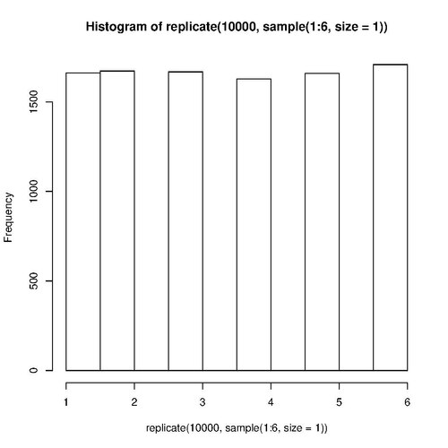
Uniform distribution
Because each face of a die is equally likely to appear on top, rolling a die many times generates the uniform distribution.[60] This example displays a histogram of a die rolled 10,000 times:
hist( replicate( 10000, sample( 1:6, size=1 ) ) )
The output is likely to have a flat top:
Central limit theorem
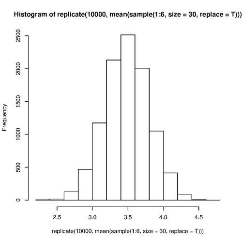
Whereas a numeric data set may have a central tendency, it also may not have a central tendency. Nonetheless, a data set of the arithmetic mean of many samples will have a central tendency to converge to the population's mean. The arithmetic mean of a sample is called the sample mean.[61] The central limit theorem states for a sample size of 30 or more, the distribution of the sample mean ([math]\displaystyle{ \bar{x} }[/math]) is approximately normally distributed, regardless of the distribution of the variable under consideration ([math]\displaystyle{ x }[/math]).[62] A histogram displaying a frequency of data point averages will show the distribution of the sample mean resembles a bell-shaped curve.
For example, rolling one die many times generates the uniform distribution. Nonetheless, rolling 30 dice and calculating each average ([math]\displaystyle{ \bar{x} }[/math]) over and over again generates a normal distribution.
R program to roll 30 dice 10,000 times and plot the frequency of averages:
hist(
    replicate(
        10000,
        mean(
            sample(
                1:6,
                size=30,
                replace=T ) ) ) )
The output is likely to have a bell shape:
Programmer created functions
To create a function object, execute the function() statement and assign the result to a name.[63] A function receives input both from global variables and input parameters (often called arguments). Objects created within the function body remain local to the function.
R program to create a function:
# The input parameters are x and y.
# The return value is a numeric double vector.
f <- function(x, y)
{
    first_expression <- x * 2
    second_expression <- y * 3
    first_expression + second_expression

    # The return statement may be omitted
    # if the last expression is unassigned.
    # This will save a few clock cycles.
}
Usage output:
> f(1, 2)
[1] 8
Function arguments are passed in by value.
If statements
R program illustrating if statements:
minimum <- function( a, b )
{
	if ( a < b )
		minimum <- a
	else
		minimum <- b

	return( minimum )
}

maximum <- function( a, b )
{
	if ( a > b )
		maximum <- a
	else
		maximum <- b

	return( maximum )
}

range <- function( a, b, c )
{
	range <-
		maximum( a, maximum( b, c ) ) -
		minimum( a, minimum( b, c ) )

	return( range )
}

range( 10, 4, 7 )
Output:
[1] 6
Generic functions
R supports generic functions. They act differently depending on the classes of the arguments passed in. The process is to dispatch the method specific to the set of classes. A common implementation is R's print() function. It can print almost every class of object. For example, print(objectName).[64]
Packages

The R package is a collection of functions, documentation, and data that expand R.[65] As examples: packages add output features to more graphical devices, transform features to import and export data, and report features such as RMarkdown, knitr and Sweave. Easy package installation and use have contributed to the language's adoption in data science.[66]
Multiple packages are included with the basic installation. Additional packages are available on repositories: CRAN, R-Forge, Omegahat, and GitHub.
The Task Views on the CRAN website lists packages in fields including finance, genetics, high-performance computing, machine learning, medical imaging, meta-analysis, social sciences, and spatial statistics.
The bioconductor project provides packages for genomic data analysis, complementary DNA, microarray, and high-throughput sequencing methods.
Packages add the capability to interface with standalone, interactive graphics.[67]
Packages add the capability to implement various statistical techniques: linear, generalized linear and nonlinear modeling, classical statistical tests, spatial analysis, time-series analysis, and clustering.
The Tidyverse package is organized to have a common interface. Each function in the package is designed to couple together all the other functions in the package.[65]
Installing a package occurs only once. To install tidyverse:[65]
> install.packages( "tidyverse" )
To instantiate the functions, data, and documentation of a package, execute the library() function. To instantiate tidyverse:[lower-alpha 4]
> library( tidyverse )
Interfaces
R comes installed with a command line console. Available for installation are various integrated development environments (IDE). IDEs for R include R.app (OSX/macOS only), Rattle GUI, R Commander, RKWard, RStudio, and Tinn-R.
General purpose IDEs that support R include Eclipse via the StatET plugin and Visual Studio via R Tools for Visual Studio.
Editors that support R include Emacs, Vim via the Nvim-R plugin, Kate, LyX via Sweave, WinEdt (website), and Jupyter (website).
Scripting languages that support R include Python (website), Perl (website), Ruby (source code), F# (website), and Julia (source code).
General purpose programming languages that support R include Java via the Rserve socket server, and .NET C# (website).
Statistical frameworks which use R in the background include Jamovi and JASP.
Implementations
The main R implementation is written primarily in C, Fortran, and R itself. Other implementations include:
- pretty quick R (pqR), by Radford M. Neal, attempts to improve memory management.
- Renjin is an implementation of R for the Java Virtual Machine.
- CXXR and Riposte[68] are implementations of R written in C++.
- Oracle's FastR is an implementation of R, built on GraalVM.
- TIBCO Software, creator of S-PLUS, wrote TERR — an R implementation to integrate with Spotfire.[69]
Microsoft R Open (MRO) was a R implementation. As of 30 June 2021, Microsoft started to phase out MRO in favor of the CRAN distribution.[70]
Community
The R community hosts many conferences and in-person meetups. These groups include:
- UseR!: an annual international R user conference (website)
- Directions in Statistical Computing (DSC) (website)
- R-Ladies: an organization to promote gender diversity in the R community (website)
- SatRdays: R-focused conferences held on Saturdays (website)
- R Conference (website)
- Posit::conf (formerly known as Rstudio::conf) (website)
The R Journal
The R Journal is an open access, refereed journal of the R project. It features short to medium-length articles on the use and development of R, including packages, programming tips, CRAN news, and foundation news.
Commercial support
Although R is an open-source project, some companies provide commercial support:
- Revolution Analytics provides commercial support for Revolution R.
- Oracle provides commercial support for the Big Data Appliance, which integrates R into its other products.
- IBM provides commercial support for in-Hadoop execution of R.
See also
- Comparison of numerical-analysis software
- Comparison of statistical packages
- List of numerical-analysis software
- List of statistical software
- Rmetrics
Notes
- ↑ The format of the regression equation differs from the algebraic format of [math]\displaystyle{ y = ax + b }[/math]. The y-intercept is placed first, and all of the independent variables are appended to the right.
- ↑ This may display to standard error a warning message that the summary may be unreliable. Nonetheless, the output of 1 is correct.
- ↑ To retrieve the value of an array of length one, the index subscript is optional.
- ↑ This displays to standard error a listing of all the packages that tidyverse depends upon. It may also display two errors showing conflict. The errors may be ignored.
References
- ↑ 1.0 1.1 1.2 Morandat, Frances; Hill, Brandon; Osvald, Leo; Vitek, Jan (11 June 2012). "Evaluating the design of the R language: objects and functions for data analysis". European Conference on Object-Oriented Programming 2012: 104–131. doi:10.1007/978-3-642-31057-7_6. https://doi.org/10.1007/978-3-642-31057-7_6. Retrieved 2016-05-17.
- ↑ 2.0 2.1 "R - Free Software Directory". https://directory.fsf.org/wiki/R#tab=Details.
- ↑ "R scripts". http://mercury.webster.edu/aleshunas/R_learning_infrastructure/R%20scripts.html.
- ↑ "R Data Format Family (.rdata, .rda)". 2017-06-09. https://www.loc.gov/preservation/digital/formats/fdd/fdd000470.shtml.
- ↑ 5.0 5.1 Hornik, Kurt; The R Core Team (2022-04-12). "R FAQ". 3.3 What are the differences between R and S?. https://cran.r-project.org/doc/FAQ/R-FAQ.html#What-are-the-differences-between-R-and-S_003f.
- ↑ "Introduction". The Julia Manual. https://docs.julialang.org/en/stable/manual/introduction/#man-introduction-1.
- ↑ Giorgi, Federico M.; Ceraolo, Carmine; Mercatelli, Daniele (2022-04-27). "The R Language: An Engine for Bioinformatics and Data Science" (in en). Life 12 (5): 648. doi:10.3390/life12050648. PMID 35629316. Bibcode: 2022Life...12..648G.
- ↑ "R: Contributors". https://www.r-project.org/contributors.html.
- ↑ "R: The R Foundation". https://www.r-project.org/foundation/.
- ↑ Ihaka, Ross. "The R Project: A Brief History and Thoughts About the Future". p. 12. https://www.stat.auckland.ac.nz/~ihaka/downloads/Otago.pdf.
- ↑ Hornik, Kurt; The R Core Team (2022-04-12). "R FAQ". 2.13 What is the R Foundation?. https://cran.r-project.org/doc/FAQ/R-FAQ.html#Why-is-R-named-R_003f.
- ↑ Ihaka, Ross. "R: Past and Future History". p. 4. https://www.stat.auckland.ac.nz/~ihaka/downloads/Interface98.pdf.
- ↑ Maechler, Martin (1997-04-01). ""R-announce", "R-help", "R-devel" : 3 mailing lists for R". https://stat.ethz.ch/pipermail/r-announce/1997/000000.html.
- ↑ Ihaka, Ross (1997-12-05). "New R Version for Unix". https://stat.ethz.ch/pipermail/r-announce/1997/000014.html.
- ↑ Ihaka, Ross. "The R Project: A Brief History and Thoughts About the Future". p. 18. https://www.stat.auckland.ac.nz/~ihaka/downloads/Otago.pdf.
- ↑ 16.0 16.1 Hornik, Kurt (2012). "The Comprehensive R Archive Network" (in en). WIREs Computational Statistics 4 (4): 394–398. doi:10.1002/wics.1212. ISSN 1939-5108. https://onlinelibrary.wiley.com/doi/10.1002/wics.1212.
- ↑ , Wikidata Q101068595.
- ↑ "The Status of CRAN Mirrors". https://cran.r-project.org/mirmon_report.html.
- ↑ "CRAN - Contributed Packages". https://cran.r-project.org/web/packages/index.html.
- ↑ 20.0 20.1 Hornik, Kurt; R Core Team (2022-04-12). "R FAQ". 2.1 What is R?. https://cran.r-project.org/doc/FAQ/R-FAQ.html#What-is-R_003f.
- ↑ 21.0 21.1 21.2 Weiss, Neil A. (2002). Elementary Statistics, Fifth Edition. Addison-Wesley. p. 90. ISBN 0-201-71058-7.
- ↑ 22.0 22.1 Weiss, Neil A. (2002). Elementary Statistics, Fifth Edition. Addison-Wesley. p. 105. ISBN 0-201-71058-7.
- ↑ Weiss, Neil A. (2002). Elementary Statistics, Fifth Edition. Addison-Wesley. p. 155. ISBN 0-201-71058-7.
- ↑ Weiss, Neil A. (2002). Elementary Statistics, Fifth Edition. Addison-Wesley. p. 146. ISBN 0-201-71058-7.
- ↑ Weiss, Neil A. (2002). Elementary Statistics, Fifth Edition. Addison-Wesley. p. 148. ISBN 0-201-71058-7.
- ↑ Weiss, Neil A. (2002). Elementary Statistics, Fifth Edition. Addison-Wesley. p. 156. ISBN 0-201-71058-7.
- ↑ Weiss, Neil A. (2002). Elementary Statistics, Fifth Edition. Addison-Wesley. p. 157. ISBN 0-201-71058-7.
- ↑ Weiss, Neil A. (2002). Elementary Statistics, Fifth Edition. Addison-Wesley. p. 170. ISBN 0-201-71058-7.
- ↑ Weiss, Neil A. (2002). Elementary Statistics, Fifth Edition. Addison-Wesley. p. 175. ISBN 0-201-71058-7. "The coefficient of determination always lies between 0 and 1 ..."
- ↑ Weiss, Neil A. (2002). Elementary Statistics, Fifth Edition. Addison-Wesley. p. 175. ISBN 0-201-71058-7.
- ↑ Grolemund, Garrett (2014). Hands-On Programming with R. O'Reilly. p. 4. ISBN 978-1-449-35901-0.
- ↑ Grolemund, Garrett (2014). Hands-On Programming with R. O'Reilly. p. 20. ISBN 978-1-449-35901-0. "An R script is just a plain text file that you save R code in."
- ↑ Grolemund, Garrett (2014). Hands-On Programming with R. O'Reilly. p. 7. ISBN 978-1-449-35901-0.
- ↑ Grolemund, Garrett (2014). Hands-On Programming with R. O'Reilly. p. 8. ISBN 978-1-449-35901-0.
- ↑ Grolemund, Garrett (2014). Hands-On Programming with R. O'Reilly. p. 37. ISBN 978-1-449-35901-0.
- ↑ Grolemund, Garrett (2014). Hands-On Programming with R. O'Reilly. p. 38. ISBN 978-1-449-35901-0.
- ↑ 37.0 37.1 Grolemund, Garrett (2014). Hands-On Programming with R. O'Reilly. p. 10. ISBN 978-1-449-35901-0.
- ↑ 38.0 38.1 38.2 Grolemund, Garrett (2014). Hands-On Programming with R. O'Reilly. p. 39. ISBN 978-1-449-35901-0.
- ↑ 39.0 39.1 39.2 Grolemund, Garrett (2014). Hands-On Programming with R. O'Reilly. p. 42. ISBN 978-1-449-35901-0.
- ↑ Grolemund, Garrett (2014). Hands-On Programming with R. O'Reilly. p. 81. ISBN 978-1-449-35901-0.
- ↑ 41.0 41.1 Grolemund, Garrett (2014). Hands-On Programming with R. O'Reilly. p. 41. ISBN 978-1-449-35901-0.
- ↑ Grolemund, Garrett (2014). Hands-On Programming with R. O'Reilly. p. 49. ISBN 978-1-449-35901-0.
- ↑ Grolemund, Garrett (2014). Hands-On Programming with R. O'Reilly. p. 50. ISBN 978-1-449-35901-0.
- ↑ Weiss, Neil A. (2002). Elementary Statistics, Fifth Edition. Addison-Wesley. p. 25. ISBN 0-201-71058-7.
- ↑ Weiss, Neil A. (2002). Elementary Statistics, Fifth Edition. Addison-Wesley. p. 23. ISBN 0-201-71058-7.
- ↑ Weiss, Neil A. (2002). Elementary Statistics, Fifth Edition. Addison-Wesley. p. 24. ISBN 0-201-71058-7.
- ↑ Grolemund, Garrett (2014). Hands-On Programming with R. O'Reilly. p. 55. ISBN 978-1-449-35901-0. "Data frames are the two-dimensional version of a list."
- ↑ Grolemund, Garrett (2014). Hands-On Programming with R. O'Reilly. p. 55. ISBN 978-1-449-35901-0. "They are far and away the most useful storage structure for data analysis[.]"
- ↑ 49.0 49.1 Grolemund, Garrett (2014). Hands-On Programming with R. O'Reilly. p. 173. ISBN 978-1-449-35901-0.
- ↑ 50.0 50.1 Grolemund, Garrett (2014). Hands-On Programming with R. O'Reilly. p. 185. ISBN 978-1-449-35901-0.
- ↑ Grolemund, Garrett (2014). Hands-On Programming with R. O'Reilly. p. 165. ISBN 978-1-449-35901-0.
- ↑ Grolemund, Garrett (2014). Hands-On Programming with R. O'Reilly. p. 69. ISBN 978-1-449-35901-0.
- ↑ Grolemund, Garrett (2014). Hands-On Programming with R. O'Reilly. p. 80. ISBN 978-1-449-35901-0.
- ↑ Grolemund, Garrett (2014). Hands-On Programming with R. O'Reilly. p. 77. ISBN 978-1-449-35901-0.
- ↑ 55.0 55.1 Grolemund, Garrett (2014). Hands-On Programming with R. O'Reilly. p. 16. ISBN 978-1-449-35901-0.
- ↑ Grolemund, Garrett (2014). Hands-On Programming with R. O'Reilly. p. 29. ISBN 978-1-449-35901-0.
- ↑ Grolemund, Garrett (2014). Hands-On Programming with R. O'Reilly. p. 13. ISBN 978-1-449-35901-0.
- ↑ 58.0 58.1 Grolemund, Garrett (2014). Hands-On Programming with R. O'Reilly. p. 14. ISBN 978-1-449-35901-0.
- ↑ Schach, Stephen R. (1990). Software Engineering. Aksen Associates Incorporated Publishers. p. 231. ISBN 0-256-08515-3.
- ↑ Downing, Douglas; Clark, Jeffrey (2003). Business Statistics. Barron's. p. 163. ISBN 0-7641-1983-4.
- ↑ Weiss, Neil A. (2002). Elementary Statistics, Fifth Edition. Addison-Wesley. p. 95. ISBN 0-201-71058-7.
- ↑ Weiss, Neil A. (2002). Elementary Statistics, Fifth Edition. Addison-Wesley. p. 314. ISBN 0-201-71058-7.
- ↑ Grolemund, Garrett (2014). Hands-On Programming with R. O'Reilly. p. 17. ISBN 978-1-449-35901-0.
- ↑ R Core Team. "Print Values". R Foundation for Statistical Computing. https://stat.ethz.ch/R-manual/R-devel/library/base/html/print.html.
- ↑ 65.0 65.1 65.2 Wickham, Hadley; Cetinkaya-Rundel, Mine; Grolemund, Garrett (2023). R for Data Science, Second Edition. O'Reilly. p. xvii. ISBN 978-1-492-09740-2.
- ↑ Chambers, John M. (2020). "S, R, and Data Science" (in en). The R Journal 12 (1): 462–476. doi:10.32614/RJ-2020-028. ISSN 2073-4859. https://journal.r-project.org/archive/2020/RJ-2020-028/index.html. "The R language and related software play a major role in computing for data science. ... R packages provide tools for a wide range of purposes and users.".
- ↑ Lewin-Koh, Nicholas (7 January 2015). "CRAN Task View: Graphic Displays & Dynamic Graphics & Graphic Devices & Visualization". https://cran.r-project.org/web/views/Graphics.html. "There are several efforts to implement interactive graphics systems that interface well with R."
- ↑ Talbot, Justin; DeVito, Zachary; Hanrahan, Pat (1 January 2012). "Riposte: A trace-driven compiler and parallel VM for vector code in R". Proceedings of the 21st international conference on Parallel architectures and compilation techniques. ACM. pp. 43–52. doi:10.1145/2370816.2370825. ISBN 9781450311823.
- ↑ Jackson, Joab (16 May 2013). TIBCO offers free R to the enterprise. PC World. Retrieved 20 July 2015.
- ↑ "Looking to the future for R in Azure SQL and SQL Server". 30 June 2021. https://cloudblogs.microsoft.com/sqlserver/2021/06/30/looking-to-the-future-for-r-in-azure-sql-and-sql-server/.
External links
- of the R project
- R Technical Papers
- Free Software Foundation
- R FAQ
 |  |

