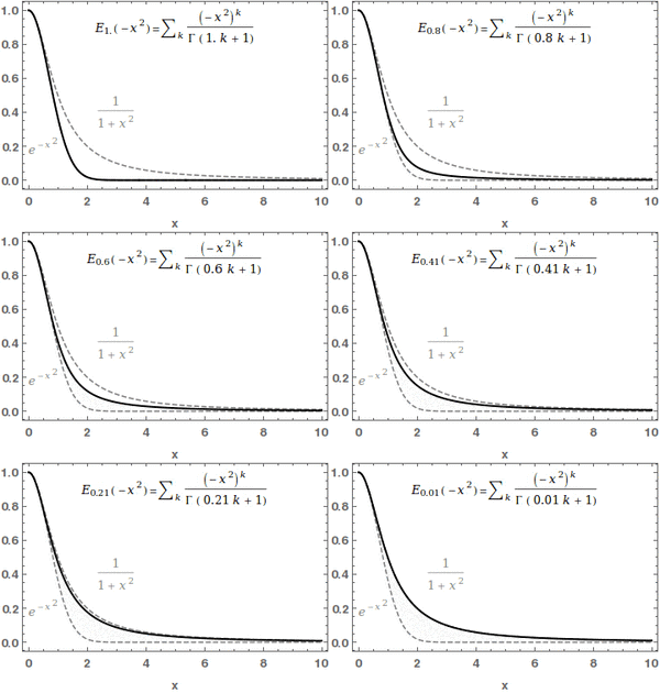
Mittag-Leffler function

Short description: Mathematical function

The Mittag-Leffler function can be used to interpolate continuously between a Gaussian and a Lorentzian function.

In mathematics, the Mittag-Leffler function [math]\displaystyle{ E_{\alpha,\beta} }[/math] is a special function, a complex function which depends on two complex parameters [math]\displaystyle{ \alpha }[/math] and [math]\displaystyle{ \beta }[/math]. It may be defined by the following series when the real part of [math]\displaystyle{ \alpha }[/math] is strictly positive:

[math]\displaystyle{ E_{\alpha, \beta} (z) = \sum_{k=0}^\infty \frac{z^k}{\Gamma(\alpha k + \beta)}, }[/math]

where [math]\displaystyle{ \Gamma(x) }[/math] is the gamma function. When [math]\displaystyle{ \beta=1 }[/math], it is abbreviated as [math]\displaystyle{ E_\alpha(z) = E_{\alpha,1}(z) }[/math]. For [math]\displaystyle{ \alpha=0 }[/math], the series above equals the Taylor expansion of the geometric series and consequently [math]\displaystyle{ E_{0,\beta}(z)=\frac{1}{\Gamma(\beta)}\frac{1}{1-z} }[/math].

In the case [math]\displaystyle{ \alpha }[/math] and [math]\displaystyle{ \beta }[/math] are real and positive, the series converges for all values of the argument [math]\displaystyle{ z }[/math], so the Mittag-Leffler function is an entire function. This function is named after Gösta Mittag-Leffler. This class of functions are important in the theory of the fractional calculus.

For [math]\displaystyle{ \alpha \gt 0 }[/math], the Mittag-Leffler function [math]\displaystyle{ E_{\alpha,1}(z) }[/math] is an entire function of order [math]\displaystyle{ 1/\alpha }[/math], and is in some sense the simplest entire function of its order.

The Mittag-Leffler function satisfies the recurrence property (Theorem 5.1 of )

[math]\displaystyle{ E_{\alpha,\beta}(z)=\frac{1}{z}E_{\alpha,\beta-\alpha}(z)-\frac{1}{z \Gamma(\beta-\alpha)}, }[/math]

from which the following Poincaré asymptotic expansion holds : for [math]\displaystyle{ 0\lt \alpha\lt 2 }[/math] and [math]\displaystyle{ \mu }[/math] real such that [math]\displaystyle{ \frac{\pi\alpha}{2} \lt \mu \lt \min(\pi, \pi\alpha) }[/math] then for all [math]\displaystyle{ N\in\mathbb{N}^*, N\neq 1 }[/math], we can show the following asymptotic expansions (Section 6. of ):

-as [math]\displaystyle{ \,|z|\to+\infty, |\text{arg}(z)|\leq \mu }[/math]:

[math]\displaystyle{ E_{\alpha}(z) = \frac{1}{\alpha} \exp(z^{\frac{1}{\alpha}}) - \sum\limits_{k=1}^{N} \frac{1}{z^k\, \Gamma(1-\alpha k)} + O\left(\frac{1}{z^{N+1}}\right) }[/math],

-and as [math]\displaystyle{ \,|z|\to+\infty, \mu\leq|\text{arg}(z)|\leq\pi }[/math]:

[math]\displaystyle{ E_{\alpha}(z) = - \sum\limits_{k=1}^N \frac{1}{z^k\Gamma(1-\alpha k)} + O\left(\frac{1}{z^{N+1}}\right) }[/math],

where we used the notation [math]\displaystyle{ E_{\alpha}(z) = E_{\alpha, 1}(z) }[/math].

Special cases

For [math]\displaystyle{ \alpha=0,1/2,1,2 }[/math] we find: (Section 2 of )

Error function:

[math]\displaystyle{ E_{\frac{1}{2}}(z) = \exp(z^2)\operatorname{erfc}(-z). }[/math]

The sum of a geometric progression:

[math]\displaystyle{ E_{0}(z) = \sum_{k=0}^\infty z^k = \frac{1}{1-z},\, |z|\lt 1. }[/math]

Exponential function:

[math]\displaystyle{ E_{1}(z) = \sum_{k=0}^\infty \frac{z^k}{\Gamma (k + 1)} = \sum_{k=0}^\infty \frac{z^k}{k!} = \exp(z). }[/math]

Hyperbolic cosine:

[math]\displaystyle{ E_{2}(z) = \cosh(\sqrt{z}), \text{ and } E_{2}(-z^2) = \cos(z). }[/math]

For [math]\displaystyle{ \beta=2 }[/math], we have

[math]\displaystyle{ E_{1,2}(z) = \frac{e^z-1}{z}, }[/math]

[math]\displaystyle{ E_{2,2}(z) = \frac{\sinh(\sqrt{z})}{\sqrt{z}}. }[/math]

For [math]\displaystyle{ \alpha=0,1,2 }[/math], the integral

[math]\displaystyle{ \int_0^z E_{\alpha}(-s^2) \, {\mathrm d}s }[/math]

gives, respectively: [math]\displaystyle{ \arctan(z) }[/math], [math]\displaystyle{ \tfrac{\sqrt{\pi}}{2}\operatorname{erf}(z) }[/math], [math]\displaystyle{ \sin(z) }[/math].

Mittag-Leffler's integral representation

The integral representation of the Mittag-Leffler function is (Section 6 of )

[math]\displaystyle{ E_{\alpha,\beta}(z)=\frac{1}{2\pi i}\oint_C \frac{t^{\alpha-\beta}e^t}{t^\alpha-z} \, dt, \Re(\alpha)\gt 0, \Re(\beta)\gt 0, }[/math]

where the contour [math]\displaystyle{ C }[/math] starts and ends at [math]\displaystyle{ -\infty }[/math] and circles around the singularities and branch points of the integrand.

Related to the Laplace transform and Mittag-Leffler summation is the expression (Eq (7.5) of with [math]\displaystyle{ m=0 }[/math])

[math]\displaystyle{ \int_0^{\infty}e^{-t z} t^{\beta-1} E_{\alpha,\beta}(\pm r\, t^\alpha) \,dt = \frac{z^{\alpha-\beta}}{z^{\alpha}\mp r}, \Re(z)\gt 0, \Re(\alpha)\gt 0, \Re(\beta)\gt 0. }[/math]

Applications of Mittag-Leffler function

One of the applications of the Mittag-Leffler function is in modeling fractional order viscoelastic materials. Experimental investigations into the time-dependent relaxation behavior of viscoelastic materials are characterized by a very fast decrease of the stress at the beginning of the relaxation process and an extremely slow decay for large times. It can even take a long time before a constant asymptotic value is reached. Therefore, a lot of Maxwell elements are required to describe relaxation behavior with sufficient accuracy. This ends in a difficult optimization problem in order to identify a large number of material parameters. On the other hand, over the years, the concept of fractional derivatives has been introduced to the theory of viscoelasticity. Among these models, the fractional Zener model was found to be very effective to predict the dynamic nature of rubber-like materials with only a small number of material parameters. The solution of the corresponding constitutive equation leads to a relaxation function of the Mittag-Leffler type. It is defined by the power series with negative arguments. This function represents all essential properties of the relaxation process under the influence of an arbitrary and continuous signal with a jump at the origin.

See also

• Mittag-Leffler summation
• Mittag-Leffler distribution
• Fox–Wright function
• Prabhakar function

Notes

• R Package 'MittagLeffleR' by Gurtek Gill, Peter Straka. Implements the Mittag-Leffler function, distribution, random variate generation, and estimation.

References

• Mittag-Leffler, M.G.: Sur la nouvelle fonction E(x). C. R. Acad. Sci. Paris 137, 554–558 (1903)
• Mittag-Leffler, M.G.: Sopra la funzione E˛.x/. Rend. R. Acc. Lincei, (Ser. 5) 13, 3–5 (1904)
• Gorenflo R., Kilbas A.A., Mainardi F., Rogosin S.V., Mittag-Leffler Functions, Related Topics and Applications (Springer, New York, 2014) 443 pages ISBN 978-3-662-43929-6
• Igor Podlubny (1998). "chapter 1". Fractional Differential Equations. An Introduction to Fractional Derivatives, Fractional Differential Equations, Some Methods of Their Solution and Some of Their Applications. Mathematics in Science and Engineering. Academic Press. ISBN 0-12-558840-2. 
• Kai Diethelm (2010). "chapter 4". The analysis of fractional differential equations: an application-oriented exposition using differential operators of Caputo type. Lecture Notes in Mathematics. Heidelberg and New York: Springer-Verlag. ISBN 978-3-642-14573-5. 

External links

• Mittag-Leffler function: MATLAB code
• Mittag-Leffler and stable random numbers: Continuous-time random walks and stochastic solution of space-time fractional diffusion equations

References

- ↑ 1.0 1.1 1.2 1.3 1.4 1.5 Saxena, R. K.; Mathai, A. M.; Haubold, H. J. (2009-09-01). "Mittag-Leffler Functions and Their Applications". arXiv:0909.0230 [math.CA].
- ↑ Weisstein, Eric W.. "Mittag-Leffler Function" (in en). http://mathworld.wolfram.com/Mittag-LefflerFunction.html.
- ↑ Pritz, T. (2003). Five-parameter fractional derivative model for polymeric damping materials. Journal of Sound and Vibration, 265(5), 935-952.
- ↑ Nonnenmacher, T. F., & Glöckle, W. G. (1991). A fractional model for mechanical stress relaxation. Philosophical magazine letters, 64(2), 89-93.