Test functions for optimization
In applied mathematics, test functions, known as artificial landscapes, are useful to evaluate characteristics of optimization algorithms, such as:
- Convergence rate.
- Precision.
- Robustness.
- General performance.
Here some test functions are presented with the aim of giving an idea about the different situations that optimization algorithms have to face when coping with these kinds of problems. In the first part, some objective functions for single-objective optimization cases are presented. In the second part, test functions with their respective Pareto fronts for multi-objective optimization problems (MOP) are given.
The artificial landscapes presented herein for single-objective optimization problems are taken from Bäck,[1] Haupt et al.[2] and from Rody Oldenhuis software.[3] Given the number of problems (55 in total), just a few are presented here.
The test functions used to evaluate the algorithms for MOP were taken from Deb,[4] Binh et al.[5] and Binh.[6] The software developed by Deb can be downloaded,[7] which implements the NSGA-II procedure with GAs, or the program posted on Internet,[8] which implements the NSGA-II procedure with ES.
Just a general form of the equation, a plot of the objective function, boundaries of the object variables and the coordinates of global minima are given herein.
Test functions for single-objective optimization
| Name | Plot | Formula | Global minimum | Search domain |
|---|---|---|---|---|
| Rastrigin function | 
|
[math]\displaystyle{ f(\mathbf{x}) = A n + \sum_{i=1}^n \left[x_i^2 - A\cos(2 \pi x_i)\right] }[/math]
[math]\displaystyle{ \text{where: } A=10 }[/math] |
[math]\displaystyle{ f(0, \dots, 0) = 0 }[/math] | [math]\displaystyle{ -5.12\le x_{i} \le 5.12 }[/math] |
| Ackley function | 
|
[math]\displaystyle{ f(x,y) = -20\exp\left[-0.2\sqrt{0.5\left(x^{2}+y^{2}\right)}\right] }[/math]
[math]\displaystyle{ -\exp\left[0.5\left(\cos 2\pi x + \cos 2\pi y \right)\right] + e + 20 }[/math] |
[math]\displaystyle{ f(0,0) = 0 }[/math] | [math]\displaystyle{ -5\le x,y \le 5 }[/math] |
| Sphere function | 
|
[math]\displaystyle{ f(\boldsymbol{x}) = \sum_{i=1}^{n} x_{i}^{2} }[/math] | [math]\displaystyle{ f(x_{1}, \dots, x_{n}) = f(0, \dots, 0) = 0 }[/math] | [math]\displaystyle{ -\infty \le x_{i} \le \infty }[/math], [math]\displaystyle{ 1 \le i \le n }[/math] |
| Rosenbrock function | 
|
[math]\displaystyle{ f(\boldsymbol{x}) = \sum_{i=1}^{n-1} \left[ 100 \left(x_{i+1} - x_{i}^{2}\right)^{2} + \left(1 - x_{i}\right)^{2}\right] }[/math] | [math]\displaystyle{ \text{Min} = \begin{cases} n=2 & \rightarrow \quad f(1,1) = 0, \\ n=3 & \rightarrow \quad f(1,1,1) = 0, \\ n\gt 3 & \rightarrow \quad f(\underbrace{1,\dots,1}_{n \text{ times}}) = 0 \\ \end{cases} }[/math] | [math]\displaystyle{ -\infty \le x_{i} \le \infty }[/math], [math]\displaystyle{ 1 \le i \le n }[/math] |
| Beale function | 
|
[math]\displaystyle{ f(x,y) = \left( 1.5 - x + xy \right)^{2} + \left( 2.25 - x + xy^{2}\right)^{2} }[/math]
[math]\displaystyle{ + \left(2.625 - x+ xy^{3}\right)^{2} }[/math] |
[math]\displaystyle{ f(3, 0.5) = 0 }[/math] | [math]\displaystyle{ -4.5 \le x,y \le 4.5 }[/math] |
| Goldstein–Price function | 
|
[math]\displaystyle{ f(x,y) = \left[1+\left(x+y+1\right)^{2}\left(19-14x+3x^{2}-14y+6xy+3y^{2}\right)\right] }[/math]
[math]\displaystyle{ \left[30+\left(2x-3y\right)^{2}\left(18-32x+12x^{2}+48y-36xy+27y^{2}\right)\right] }[/math] |
[math]\displaystyle{ f(0, -1) = 3 }[/math] | [math]\displaystyle{ -2 \le x,y \le 2 }[/math] |
| Booth function | 
|
[math]\displaystyle{ f(x,y) = \left( x + 2y -7\right)^{2} + \left(2x +y - 5\right)^{2} }[/math] | [math]\displaystyle{ f(1,3) = 0 }[/math] | [math]\displaystyle{ -10 \le x,y \le 10 }[/math] |
| Bukin function N.6 | 
|
[math]\displaystyle{ f(x,y) = 100\sqrt{\left|y - 0.01x^{2}\right|} + 0.01 \left|x+10 \right|.\quad }[/math] | [math]\displaystyle{ f(-10,1) = 0 }[/math] | [math]\displaystyle{ -15\le x \le -5 }[/math], [math]\displaystyle{ -3\le y \le 3 }[/math] |
| Matyas function | 
|
[math]\displaystyle{ f(x,y) = 0.26 \left( x^{2} + y^{2}\right) - 0.48 xy }[/math] | [math]\displaystyle{ f(0,0) = 0 }[/math] | [math]\displaystyle{ -10\le x,y \le 10 }[/math] |
| Lévi function N.13 | 
|
[math]\displaystyle{ f(x,y) = \sin^{2} 3\pi x + \left(x-1\right)^{2}\left(1+\sin^{2} 3\pi y\right) }[/math]
[math]\displaystyle{ +\left(y-1\right)^{2}\left(1+\sin^{2} 2\pi y\right) }[/math] |
[math]\displaystyle{ f(1,1) = 0 }[/math] | [math]\displaystyle{ -10\le x,y \le 10 }[/math] |
| Himmelblau's function | 
|
[math]\displaystyle{ f(x, y) = (x^2+y-11)^2 + (x+y^2-7)^2.\quad }[/math] | [math]\displaystyle{ \text{Min} = \begin{cases} f\left(3.0, 2.0\right) & = 0.0 \\ f\left(-2.805118, 3.131312\right) & = 0.0 \\ f\left(-3.779310, -3.283186\right) & = 0.0 \\ f\left(3.584428, -1.848126\right) & = 0.0 \\ \end{cases} }[/math] | [math]\displaystyle{ -5\le x,y \le 5 }[/math] |
| Three-hump camel function | 
|
[math]\displaystyle{ f(x,y) = 2x^{2} - 1.05x^{4} + \frac{x^{6}}{6} + xy + y^{2} }[/math] | [math]\displaystyle{ f(0,0) = 0 }[/math] | [math]\displaystyle{ -5\le x,y \le 5 }[/math] |
| Easom function | 
|
[math]\displaystyle{ f(x,y) = -\cos \left(x\right)\cos \left(y\right) \exp\left(-\left(\left(x-\pi\right)^{2} + \left(y-\pi\right)^{2}\right)\right) }[/math] | [math]\displaystyle{ f(\pi , \pi) = -1 }[/math] | [math]\displaystyle{ -100\le x,y \le 100 }[/math] |
| Cross-in-tray function | 
|
[math]\displaystyle{ f(x,y) = -0.0001 \left[ \left| \sin x \sin y \exp \left(\left|100 - \frac{\sqrt{x^{2} + y^{2}}}{\pi} \right|\right)\right| + 1 \right]^{0.1} }[/math] | [math]\displaystyle{ \text{Min} = \begin{cases} f\left(1.34941, -1.34941\right) & = -2.06261 \\ f\left(1.34941, 1.34941\right) & = -2.06261 \\ f\left(-1.34941, 1.34941\right) & = -2.06261 \\ f\left(-1.34941,-1.34941\right) & = -2.06261 \\ \end{cases} }[/math] | [math]\displaystyle{ -10\le x,y \le 10 }[/math] |
| Eggholder function[9][10] | 
|
[math]\displaystyle{ f(x,y) = - \left(y+47\right) \sin \sqrt{\left|\frac{x}{2}+\left(y+47\right)\right|} - x \sin \sqrt{\left|x - \left(y + 47 \right)\right|} }[/math] | [math]\displaystyle{ f(512, 404.2319) = -959.6407 }[/math] | [math]\displaystyle{ -512\le x,y \le 512 }[/math] |
| Hölder table function | 
|
[math]\displaystyle{ f(x,y) = - \left|\sin x \cos y \exp \left(\left|1 - \frac{\sqrt{x^{2} + y^{2}}}{\pi} \right|\right)\right| }[/math] | [math]\displaystyle{ \text{Min} = \begin{cases} f\left(8.05502, 9.66459\right) & = -19.2085 \\ f\left(-8.05502, 9.66459\right) & = -19.2085 \\ f\left(8.05502,-9.66459\right) & = -19.2085 \\ f\left(-8.05502,-9.66459\right) & = -19.2085 \end{cases} }[/math] | [math]\displaystyle{ -10\le x,y \le 10 }[/math] |
| McCormick function | 
|
[math]\displaystyle{ f(x,y) = \sin \left(x+y\right) + \left(x-y\right)^{2} - 1.5x + 2.5y + 1 }[/math] | [math]\displaystyle{ f(-0.54719,-1.54719) = -1.9133 }[/math] | [math]\displaystyle{ -1.5\le x \le 4 }[/math], [math]\displaystyle{ -3\le y \le 4 }[/math] |
| Schaffer function N. 2 | 
|
[math]\displaystyle{ f(x,y) = 0.5 + \frac{\sin^{2}\left(x^{2} - y^{2}\right) - 0.5}{\left[1 + 0.001\left(x^{2} + y^{2}\right) \right]^{2}} }[/math] | [math]\displaystyle{ f(0, 0) = 0 }[/math] | [math]\displaystyle{ -100\le x,y \le 100 }[/math] |
| Schaffer function N. 4 | 
|
[math]\displaystyle{ f(x,y) = 0.5 + \frac{\cos^{2}\left[\sin \left( \left|x^{2} - y^{2}\right|\right)\right] - 0.5}{\left[1 + 0.001\left(x^{2} + y^{2}\right) \right]^{2}} }[/math] | [math]\displaystyle{ \text{Min} = \begin{cases} f\left(0,1.25313\right) & = 0.292579 \\ f\left(0,-1.25313\right) & = 0.292579 \\ f\left(1.25313,0\right) & = 0.292579 \\ f\left(-1.25313,0\right) & = 0.292579 \end{cases} }[/math] | [math]\displaystyle{ -100\le x,y \le 100 }[/math] |
| Styblinski–Tang function | 
|
[math]\displaystyle{ f(\boldsymbol{x}) = \frac{\sum_{i=1}^{n} x_{i}^{4} - 16x_{i}^{2} + 5x_{i}}{2} }[/math] | [math]\displaystyle{ -39.16617n \lt f(\underbrace{-2.903534, \ldots, -2.903534}_{n \text{ times}} ) \lt -39.16616n }[/math] | [math]\displaystyle{ -5\le x_{i} \le 5 }[/math], [math]\displaystyle{ 1\le i \le n }[/math].. |
| Shekel function | 
|
[math]\displaystyle{
f(\vec{x}) = \sum_{i = 1}^{m} \; \left( c_{i} + \sum\limits_{j = 1}^{n} (x_{j} - a_{ji})^2 \right)^{-1}
}[/math]
or, similarly, [math]\displaystyle{ f(x_1,x_2,...,x_{n-1},x_n) = \sum_{i = 1}^{m} \; \left( c_{i} + \sum\limits_{j = 1}^{n} (x_{j} - a_{ij})^2 \right)^{-1} }[/math] |
[math]\displaystyle{ -\infty \le x_{i} \le \infty }[/math], [math]\displaystyle{ 1 \le i \le n }[/math] |
Test functions for constrained optimization
| Name | Plot | Formula | Global minimum | Search domain |
|---|---|---|---|---|
| Rosenbrock function constrained with a cubic and a line[11] | 
|
[math]\displaystyle{ f(x,y) = (1-x)^2 + 100(y-x^2)^2 }[/math],
subjected to: [math]\displaystyle{ (x-1)^3 - y + 1 \le 0 \text{ and } x + y - 2 \le 0 }[/math] |
[math]\displaystyle{ f(1.0,1.0) = 0 }[/math] | [math]\displaystyle{ -1.5\le x \le 1.5 }[/math], [math]\displaystyle{ -0.5\le y \le 2.5 }[/math] |
| Rosenbrock function constrained to a disk[12] | 
|
[math]\displaystyle{ f(x,y) = (1-x)^2 + 100(y-x^2)^2 }[/math],
subjected to: [math]\displaystyle{ x^2 + y^2 \le 2 }[/math] |
[math]\displaystyle{ f(1.0,1.0) = 0 }[/math] | [math]\displaystyle{ -1.5\le x \le 1.5 }[/math], [math]\displaystyle{ -1.5\le y \le 1.5 }[/math] |
| Mishra's Bird function - constrained[13][14] | 
|
[math]\displaystyle{ f(x,y) = \sin(y) e^{\left [(1-\cos x)^2\right]} + \cos(x) e^{\left [(1-\sin y)^2 \right]} + (x-y)^2 }[/math],
subjected to: [math]\displaystyle{ (x+5)^2 + (y+5)^2 \lt 25 }[/math] |
[math]\displaystyle{ f(-3.1302468,-1.5821422) = -106.7645367 }[/math] | [math]\displaystyle{ -10\le x \le 0 }[/math], [math]\displaystyle{ -6.5\le y \le 0 }[/math] |
| Townsend function (modified)[15] | 
|
[math]\displaystyle{ f(x,y) = -[\cos((x-0.1)y)]^2 - x \sin(3x+y) }[/math],
subjected to:[math]\displaystyle{ x^2+y^2 \lt \left[2\cos t - \frac 1 2 \cos 2t - \frac 1 4 \cos 3t - \frac 1 8 \cos 4t\right]^2 + [2\sin t]^2 }[/math] where: t = Atan2(x,y) |
[math]\displaystyle{ f(2.0052938,1.1944509) = -2.0239884 }[/math] | [math]\displaystyle{ -2.25\le x \le 2.25 }[/math], [math]\displaystyle{ -2.5\le y \le 1.75 }[/math] |
| Gomez and Levy function (modified)[16] | 
|
[math]\displaystyle{ f(x,y) = 4 x^2 - 2.1 x^4 + \frac 1 3 x^6 + xy - 4y^2 +4 y^4 }[/math],
subjected to:[math]\displaystyle{ -\sin(4 \pi x) + 2\sin^2(2 \pi y) \le 1.5 }[/math] |
[math]\displaystyle{ f(0.08984201,-0.7126564) = -1.031628453 }[/math] | [math]\displaystyle{ -1\le x \le 0.75 }[/math], [math]\displaystyle{ -1\le y \le 1 }[/math] |
| Simionescu function[17] | 
|
[math]\displaystyle{ f(x,y) = 0.1xy }[/math],
subjected to: [math]\displaystyle{ x^2+y^2\le\left[r_{T}+r_{S}\cos\left(n \arctan \frac{x}{y} \right)\right]^2 }[/math] [math]\displaystyle{ \text{where: } r_{T}=1, r_{S}=0.2 \text{ and } n = 8 }[/math] |
[math]\displaystyle{ f(\pm 0.84852813,\mp 0.84852813) = -0.072 }[/math] | [math]\displaystyle{ -1.25\le x,y \le 1.25 }[/math] |
Test functions for multi-objective optimization
| Name | Plot | Functions | Constraints | Search domain |
|---|---|---|---|---|
| Binh and Korn function:[5] | 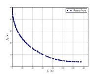
|
[math]\displaystyle{ \text{Minimize} = \begin{cases} f_{1}\left(x,y\right) = 4x^{2} + 4y^{2} \\ f_{2}\left(x,y\right) = \left(x - 5\right)^{2} + \left(y - 5\right)^{2} \\ \end{cases} }[/math] | [math]\displaystyle{ \text{s.t.} = \begin{cases} g_{1}\left(x,y\right) = \left(x - 5\right)^{2} + y^{2} \leq 25 \\ g_{2}\left(x,y\right) = \left(x - 8\right)^{2} + \left(y + 3\right)^{2} \geq 7.7 \\ \end{cases} }[/math] | [math]\displaystyle{ 0\le x \le 5 }[/math], [math]\displaystyle{ 0\le y \le 3 }[/math] |
| Chankong and Haimes function:[18] | 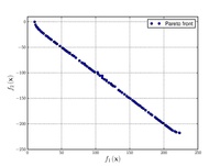
|
[math]\displaystyle{ \text{Minimize} = \begin{cases} f_{1}\left(x,y\right) = 2 + \left(x-2\right)^{2} + \left(y-1\right)^{2} \\ f_{2}\left(x,y\right) = 9x - \left(y - 1\right)^{2} \\ \end{cases} }[/math] | [math]\displaystyle{ \text{s.t.} = \begin{cases} g_{1}\left(x,y\right) = x^{2} + y^{2} \leq 225 \\ g_{2}\left(x,y\right) = x - 3y + 10 \leq 0 \\ \end{cases} }[/math] | [math]\displaystyle{ -20\le x,y \le 20 }[/math] |
| Fonseca–Fleming function:[19] | 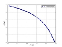
|
[math]\displaystyle{ \text{Minimize} = \begin{cases} f_{1}\left(\boldsymbol{x}\right) = 1 - \exp \left[-\sum_{i=1}^{n} \left(x_{i} - \frac{1}{\sqrt{n}} \right)^{2} \right] \\ f_{2}\left(\boldsymbol{x}\right) = 1 - \exp \left[-\sum_{i=1}^{n} \left(x_{i} + \frac{1}{\sqrt{n}} \right)^{2} \right] \\ \end{cases} }[/math] | [math]\displaystyle{ -4\le x_{i} \le 4 }[/math], [math]\displaystyle{ 1\le i \le n }[/math] | |
| Test function 4:[6] | ![Test function 4.[6]](/wiki/images/thumb/3/3c/Test_function_4_-_Binh.pdf/page1-200px-Test_function_4_-_Binh.pdf.jpg)
|
[math]\displaystyle{ \text{Minimize} = \begin{cases} f_{1}\left(x,y\right) = x^{2} - y \\ f_{2}\left(x,y\right) = -0.5x - y - 1 \\ \end{cases} }[/math] | [math]\displaystyle{ \text{s.t.} = \begin{cases} g_{1}\left(x,y\right) = 6.5 - \frac{x}{6} - y \geq 0 \\ g_{2}\left(x,y\right) = 7.5 - 0.5x - y \geq 0 \\ g_{3}\left(x,y\right) = 30 - 5x - y \geq 0 \\ \end{cases} }[/math] | [math]\displaystyle{ -7\le x,y \le 4 }[/math] |
| Kursawe function:[20] | 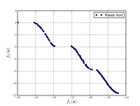
|
[math]\displaystyle{ \text{Minimize} = \begin{cases} f_{1}\left(\boldsymbol{x}\right) = \sum_{i=1}^{2} \left[-10 \exp \left(-0.2 \sqrt{x_{i}^{2} + x_{i+1}^{2}} \right) \right] \\ & \\ f_{2}\left(\boldsymbol{x}\right) = \sum_{i=1}^{3} \left[\left|x_{i}\right|^{0.8} + 5 \sin \left(x_{i}^{3} \right) \right] \\ \end{cases} }[/math] | [math]\displaystyle{ -5\le x_{i} \le 5 }[/math], [math]\displaystyle{ 1\le i \le 3 }[/math]. | |
| Schaffer function N. 1:[21] | 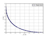
|
[math]\displaystyle{ \text{Minimize} = \begin{cases} f_{1}\left(x\right) = x^{2} \\ f_{2}\left(x\right) = \left(x-2\right)^{2} \\ \end{cases} }[/math] | [math]\displaystyle{ -A\le x \le A }[/math]. Values of [math]\displaystyle{ A }[/math] from [math]\displaystyle{ 10 }[/math] to [math]\displaystyle{ 10^{5} }[/math] have been used successfully. Higher values of [math]\displaystyle{ A }[/math] increase the difficulty of the problem. | |
| Schaffer function N. 2: | 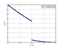
|
[math]\displaystyle{ \text{Minimize} = \begin{cases} f_{1}\left(x\right) = \begin{cases} -x, & \text{if } x \le 1 \\ x-2, & \text{if } 1 \lt x \le 3 \\ 4-x, & \text{if } 3 \lt x \le 4 \\ x-4, & \text{if } x \gt 4 \\ \end{cases} \\ f_{2}\left(x\right) = \left(x-5\right)^{2} \\ \end{cases} }[/math] | [math]\displaystyle{ -5\le x \le 10 }[/math]. | |
| Poloni's two objective function: | 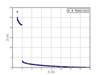
|
[math]\displaystyle{ \text{Minimize} =
\begin{cases}
f_{1}\left(x,y\right) = \left[1 + \left(A_{1} - B_{1}\left(x,y\right) \right)^{2} + \left(A_{2} - B_{2}\left(x,y\right) \right)^{2} \right] \\
f_{2}\left(x,y\right) = \left(x + 3\right)^{2} + \left(y + 1 \right)^{2} \\
\end{cases}
}[/math]
[math]\displaystyle{ \text{where} = \begin{cases} A_{1} = 0.5 \sin \left(1\right) - 2 \cos \left(1\right) + \sin \left(2\right) - 1.5 \cos \left(2\right) \\ A_{2} = 1.5 \sin \left(1\right) - \cos \left(1\right) + 2 \sin \left(2\right) - 0.5 \cos \left(2\right) \\ B_{1}\left(x,y\right) = 0.5 \sin \left(x\right) - 2 \cos \left(x\right) + \sin \left(y\right) - 1.5 \cos \left(y\right) \\ B_{2}\left(x,y\right) = 1.5 \sin \left(x\right) - \cos \left(x\right) + 2 \sin \left(y\right) - 0.5 \cos \left(y\right) \end{cases} }[/math] |
[math]\displaystyle{ -\pi\le x,y \le \pi }[/math] | |
| Zitzler–Deb–Thiele's function N. 1:[22] | 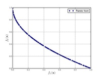
|
[math]\displaystyle{ \text{Minimize} = \begin{cases} f_{1}\left(\boldsymbol{x}\right) = x_{1} \\ f_{2}\left(\boldsymbol{x}\right) = g\left(\boldsymbol{x}\right) h \left(f_{1}\left(\boldsymbol{x}\right),g\left(\boldsymbol{x}\right)\right) \\ g\left(\boldsymbol{x}\right) = 1 + \frac{9}{29} \sum_{i=2}^{30} x_{i} \\ h \left(f_{1}\left(\boldsymbol{x}\right),g\left(\boldsymbol{x}\right)\right) = 1 - \sqrt{\frac{f_{1}\left(\boldsymbol{x}\right)}{g\left(\boldsymbol{x}\right)}} \\ \end{cases} }[/math] | [math]\displaystyle{ 0\le x_{i} \le 1 }[/math], [math]\displaystyle{ 1\le i \le 30 }[/math]. | |
| Zitzler–Deb–Thiele's function N. 2:[22] | 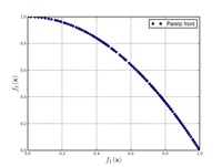
|
[math]\displaystyle{ \text{Minimize} = \begin{cases} f_{1}\left(\boldsymbol{x}\right) = x_{1} \\ f_{2}\left(\boldsymbol{x}\right) = g\left(\boldsymbol{x}\right) h \left(f_{1}\left(\boldsymbol{x}\right),g\left(\boldsymbol{x}\right)\right) \\ g\left(\boldsymbol{x}\right) = 1 + \frac{9}{29} \sum_{i=2}^{30} x_{i} \\ h \left(f_{1}\left(\boldsymbol{x}\right),g\left(\boldsymbol{x}\right)\right) = 1 - \left(\frac{f_{1}\left(\boldsymbol{x}\right)}{g\left(\boldsymbol{x}\right)}\right)^{2} \\ \end{cases} }[/math] | [math]\displaystyle{ 0\le x_{i} \le 1 }[/math], [math]\displaystyle{ 1\le i \le 30 }[/math]. | |
| Zitzler–Deb–Thiele's function N. 3:[22] | 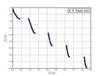
|
[math]\displaystyle{ \text{Minimize} = \begin{cases} f_{1}\left(\boldsymbol{x}\right) = x_{1} \\ f_{2}\left(\boldsymbol{x}\right) = g\left(\boldsymbol{x}\right) h \left(f_{1}\left(\boldsymbol{x}\right),g\left(\boldsymbol{x}\right)\right) \\ g\left(\boldsymbol{x}\right) = 1 + \frac{9}{29} \sum_{i=2}^{30} x_{i} \\ h \left(f_{1}\left(\boldsymbol{x}\right),g\left(\boldsymbol{x}\right)\right) = 1 - \sqrt{\frac{f_{1}\left(\boldsymbol{x}\right)}{g\left(\boldsymbol{x} \right)}} - \left(\frac{f_{1}\left(\boldsymbol{x}\right)}{g\left(\boldsymbol{x}\right)} \right) \sin \left(10 \pi f_{1} \left(\boldsymbol{x} \right) \right) \end{cases} }[/math] | [math]\displaystyle{ 0\le x_{i} \le 1 }[/math], [math]\displaystyle{ 1\le i \le 30 }[/math]. | |
| Zitzler–Deb–Thiele's function N. 4:[22] | 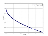
|
[math]\displaystyle{ \text{Minimize} = \begin{cases} f_{1}\left(\boldsymbol{x}\right) = x_{1} \\ f_{2}\left(\boldsymbol{x}\right) = g\left(\boldsymbol{x}\right) h \left(f_{1}\left(\boldsymbol{x}\right),g\left(\boldsymbol{x}\right)\right) \\ g\left(\boldsymbol{x}\right) = 91 + \sum_{i=2}^{10} \left(x_{i}^{2} - 10 \cos \left(4 \pi x_{i}\right) \right) \\ h \left(f_{1}\left(\boldsymbol{x}\right),g\left(\boldsymbol{x}\right)\right) = 1 - \sqrt{\frac{f_{1}\left(\boldsymbol{x}\right)}{g\left(\boldsymbol{x} \right)}} \end{cases} }[/math] | [math]\displaystyle{ 0\le x_{1} \le 1 }[/math], [math]\displaystyle{ -5\le x_{i} \le 5 }[/math], [math]\displaystyle{ 2\le i \le 10 }[/math] | |
| Zitzler–Deb–Thiele's function N. 6:[22] | 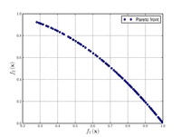
|
[math]\displaystyle{ \text{Minimize} = \begin{cases} f_{1}\left(\boldsymbol{x}\right) = 1 - \exp \left(-4x_{1}\right)\sin^{6}\left(6 \pi x_{1} \right) \\ f_{2}\left(\boldsymbol{x}\right) = g\left(\boldsymbol{x}\right) h \left(f_{1}\left(\boldsymbol{x}\right),g\left(\boldsymbol{x}\right)\right) \\ g\left(\boldsymbol{x}\right) = 1 + 9 \left[\frac{\sum_{i=2}^{10} x_{i}}{9}\right]^{0.25} \\ h \left(f_{1}\left(\boldsymbol{x}\right),g\left(\boldsymbol{x}\right)\right) = 1 - \left(\frac{f_{1}\left(\boldsymbol{x}\right)}{g\left(\boldsymbol{x} \right)}\right)^{2} \\ \end{cases} }[/math] | [math]\displaystyle{ 0\le x_{i} \le 1 }[/math], [math]\displaystyle{ 1\le i \le 10 }[/math]. | |
| Osyczka and Kundu function:[23] | 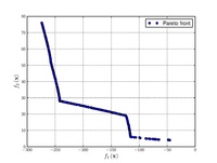
|
[math]\displaystyle{ \text{Minimize} = \begin{cases} f_{1}\left(\boldsymbol{x}\right) = -25 \left(x_{1}-2\right)^{2} - \left(x_{2}-2\right)^{2} - \left(x_{3}-1\right)^{2} - \left(x_{4}-4\right)^{2} - \left(x_{5}-1\right)^{2} \\ f_{2}\left(\boldsymbol{x}\right) = \sum_{i=1}^{6} x_{i}^{2} \\ \end{cases} }[/math] | [math]\displaystyle{ \text{s.t.} = \begin{cases} g_{1}\left(\boldsymbol{x}\right) = x_{1} + x_{2} - 2 \geq 0 \\ g_{2}\left(\boldsymbol{x}\right) = 6 - x_{1} - x_{2} \geq 0 \\ g_{3}\left(\boldsymbol{x}\right) = 2 - x_{2} + x_{1} \geq 0 \\ g_{4}\left(\boldsymbol{x}\right) = 2 - x_{1} + 3x_{2} \geq 0 \\ g_{5}\left(\boldsymbol{x}\right) = 4 - \left(x_{3}-3\right)^{2} - x_{4} \geq 0 \\ g_{6}\left(\boldsymbol{x}\right) = \left(x_{5} - 3\right)^{2} + x_{6} - 4 \geq 0 \end{cases} }[/math] | [math]\displaystyle{ 0\le x_{1},x_{2},x_{6} \le 10 }[/math], [math]\displaystyle{ 1\le x_{3},x_{5} \le 5 }[/math], [math]\displaystyle{ 0\le x_{4} \le 6 }[/math]. |
| CTP1 function (2 variables):[4][24] | ![CTP1 function (2 variables).[4]](/wiki/images/thumb/d/d4/CTP1_function_%282_variables%29.pdf/page1-200px-CTP1_function_%282_variables%29.pdf.jpg)
|
[math]\displaystyle{ \text{Minimize} = \begin{cases} f_{1}\left(x,y\right) = x \\ f_{2}\left(x,y\right) = \left(1 + y\right) \exp \left(-\frac{x}{1+y} \right) \end{cases} }[/math] | [math]\displaystyle{ \text{s.t.} = \begin{cases} g_{1}\left(x,y\right) = \frac{f_{2}\left(x,y\right)}{0.858 \exp \left(-0.541 f_{1}\left(x,y\right)\right)} \geq 1 \\ g_{2}\left(x,y\right) = \frac{f_{2}\left(x,y\right)}{0.728 \exp \left(-0.295 f_{1}\left(x,y\right)\right)} \geq 1 \end{cases} }[/math] | [math]\displaystyle{ 0\le x,y \le 1 }[/math]. |
| Constr-Ex problem:[4] | ![Constr-Ex problem.[4]](/wiki/images/thumb/6/6f/Constr-Ex_problem.pdf/page1-200px-Constr-Ex_problem.pdf.jpg)
|
[math]\displaystyle{ \text{Minimize} = \begin{cases} f_{1}\left(x,y\right) = x \\ f_{2}\left(x,y\right) = \frac{1 + y}{x} \\ \end{cases} }[/math] | [math]\displaystyle{ \text{s.t.} = \begin{cases} g_{1}\left(x,y\right) = y + 9x \geq 6 \\ g_{2}\left(x,y\right) = -y + 9x \geq 1 \\ \end{cases} }[/math] | [math]\displaystyle{ 0.1\le x \le 1 }[/math], [math]\displaystyle{ 0\le y \le 5 }[/math] |
| Viennet function: | 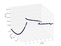
|
[math]\displaystyle{ \text{Minimize} = \begin{cases} f_{1}\left(x,y\right) = 0.5\left(x^{2} + y^{2}\right) + \sin\left(x^{2} + y^{2} \right) \\ f_{2}\left(x,y\right) = \frac{\left(3x - 2y + 4\right)^{2}}{8} + \frac{\left(x - y + 1\right)^{2}}{27} + 15 \\ f_{3}\left(x,y\right) = \frac{1}{x^{2} + y^{2} + 1} - 1.1 \exp \left(- \left(x^{2} + y^{2} \right) \right) \\ \end{cases} }[/math] | [math]\displaystyle{ -3\le x,y \le 3 }[/math]. |
References
- ↑ Bäck, Thomas (1995). Evolutionary algorithms in theory and practice : evolution strategies, evolutionary programming, genetic algorithms. Oxford: Oxford University Press. p. 328. ISBN 978-0-19-509971-3.
- ↑ Haupt, Randy L. Haupt, Sue Ellen (2004). Practical genetic algorithms with CD-Rom (2nd ed.). New York: J. Wiley. ISBN 978-0-471-45565-3.
- ↑ Oldenhuis, Rody. "Many test functions for global optimizers". Mathworks. http://www.mathworks.com/matlabcentral/fileexchange/23147-many-testfunctions-for-global-optimizers.
- ↑ 4.0 4.1 4.2 4.3 4.4 Deb, Kalyanmoy (2002) Multiobjective optimization using evolutionary algorithms (Repr. ed.). Chichester [u.a.]: Wiley. ISBN 0-471-87339-X.
- ↑ 5.0 5.1 Binh T. and Korn U. (1997) MOBES: A Multiobjective Evolution Strategy for Constrained Optimization Problems. In: Proceedings of the Third International Conference on Genetic Algorithms. Czech Republic. pp. 176–182
- ↑ 6.0 6.1 6.2 Binh T. (1999) A multiobjective evolutionary algorithm. The study cases. Technical report. Institute for Automation and Communication. Barleben, Germany
- ↑ Deb K. (2011) Software for multi-objective NSGA-II code in C. Available at URL: https://www.iitk.ac.in/kangal/codes.shtml
- ↑ Ortiz, Gilberto A.. "Multi-objective optimization using ES as Evolutionary Algorithm.". Mathworks. http://www.mathworks.com/matlabcentral/fileexchange/35824-multi-objective-optimization-using-evolution-strategies-es-as-evolutionary-algorithm-ea.
- ↑ Whitley, Darrell; Rana, Soraya; Dzubera, John; Mathias, Keith E. (1996). "Evaluating evolutionary algorithms". Artificial Intelligence (Elsevier BV) 85 (1–2): 264. doi:10.1016/0004-3702(95)00124-7. ISSN 0004-3702.
- ↑ Vanaret C. (2015) Hybridization of interval methods and evolutionary algorithms for solving difficult optimization problems. PhD thesis. Ecole Nationale de l'Aviation Civile. Institut National Polytechnique de Toulouse, France.
- ↑ Simionescu, P.A.; Beale, D. (September 29 – October 2, 2002). "New Concepts in Graphic Visualization of Objective Functions". ASME 2002 International Design Engineering Technical Conferences and Computers and Information in Engineering Conference. Montreal, Canada. pp. 891–897. http://faculty.tamucc.edu/psimionescu/PDFs/DETC02-DAC-34129.pdf. Retrieved 7 January 2017.
- ↑ "Solve a Constrained Nonlinear Problem - MATLAB & Simulink". https://www.mathworks.com/help/optim/ug/example-nonlinear-constrained-minimization.html?requestedDomain=www.mathworks.com.
- ↑ "Bird Problem (Constrained) | Phoenix Integration". http://www.phoenix-int.com/software/benchmark_report/bird_constrained.php.
- ↑ Mishra, Sudhanshu (2006). "Some new test functions for global optimization and performance of repulsive particle swarm method". MPRA Paper. https://mpra.ub.uni-muenchen.de/2718/.
- ↑ Townsend, Alex (January 2014). "Constrained optimization in Chebfun". http://www.chebfun.org/examples/opt/ConstrainedOptimization.html.
- ↑ Simionescu, P.A. (2020). "A collection of bivariate nonlinear optimisation test problems with graphical representations". International Journal of Mathematical Modelling and Numerical Optimisation 10 (4): 365–398. doi:10.1504/IJMMNO.2020.110704.
- ↑ Simionescu, P.A. (2014). Computer Aided Graphing and Simulation Tools for AutoCAD Users (1st ed.). Boca Raton, FL: CRC Press. ISBN 978-1-4822-5290-3.
- ↑ Chankong, Vira; Haimes, Yacov Y. (1983). Multiobjective decision making. Theory and methodology.. North Holland. ISBN 0-444-00710-5.
- ↑ Fonseca, C. M.; Fleming, P. J. (1995). "An Overview of Evolutionary Algorithms in Multiobjective Optimization". Evol Comput 3 (1): 1–16. doi:10.1162/evco.1995.3.1.1.
- ↑ F. Kursawe, “A variant of evolution strategies for vector optimization,” in PPSN I, Vol 496 Lect Notes in Comput Sc. Springer-Verlag, 1991, pp. 193–197.
- ↑ Schaffer, J. David (1984). "Multiple Objective Optimization with Vector Evaluated Genetic Algorithms". Proceedings of the First International Conference on Genetic Algorithms. OCLC 20004572.
- ↑ 22.0 22.1 22.2 22.3 22.4 Deb, Kalyan; Thiele, L.; Laumanns, Marco; Zitzler, Eckart (2002). "Scalable multi-objective optimization test problems". Proceedings of the 2002 Congress on Evolutionary Computation. CEC'02 (Cat. No.02TH8600). 1. pp. 825–830. doi:10.1109/CEC.2002.1007032. ISBN 0-7803-7282-4.
- ↑ Osyczka, A.; Kundu, S. (1 October 1995). "A new method to solve generalized multicriteria optimization problems using the simple genetic algorithm". Structural Optimization 10 (2): 94–99. doi:10.1007/BF01743536. ISSN 1615-1488.
- ↑ Jimenez, F.; Gomez-Skarmeta, A. F.; Sanchez, G.; Deb, K. (May 2002). "An evolutionary algorithm for constrained multi-objective optimization". Proceedings of the 2002 Congress on Evolutionary Computation. CEC'02 (Cat. No.02TH8600). 2. pp. 1133–1138. doi:10.1109/CEC.2002.1004402. ISBN 0-7803-7282-4.
 |  |

