Physics:Acoustic streaming
Acoustic streaming is a steady flow in a fluid driven by the absorption of high amplitude acoustic oscillations. This phenomenon can be observed near sound emitters, or in the standing waves within a Kundt's tube. Acoustic streaming was explained first by Lord Rayleigh in 1884.[1] It is the less-known opposite of sound generation by a flow.
There are two situations where sound is absorbed in its medium of propagation:
- during propagation in bulk flow ('Eckart streaming').[2] The attenuation coefficient is [math]\displaystyle{ \alpha=2\eta\omega^2/(3\rho c^3) }[/math], following Stokes' law (sound attenuation). This effect is more intense at elevated frequencies and is much greater in air (where attenuation occurs on a characteristic distance [math]\displaystyle{ \alpha^{-1} }[/math]~10 cm at 1 MHz) than in water ([math]\displaystyle{ \alpha^{-1} }[/math]~100 m at 1 MHz). In air it is known as the Quartz wind.
- near a boundary ('Rayleigh streaming'). Either when sound reaches a boundary, or when a boundary is vibrating in a still medium.[3] A wall vibrating parallel to itself generates a shear wave, of attenuated amplitude within the Stokes oscillating boundary layer. This effect is localised on an attenuation length of characteristic size [math]\displaystyle{ \delta=[\eta/(\rho\omega)]^{1/2} }[/math] whose order of magnitude is a few micrometres in both air and water at 1 MHz. The streaming flow generated due to the interaction of sound waves and microbubbles, elastic polymers,[4] and even biological cells[5] are examples of boundary driven acoustic streaming.
Rayleigh streaming
Consider a plane standing sound wave that corresponds to the velocity field [math]\displaystyle{ U(x,t) = v_0 \cos kx \cos \omega t = \varepsilon \cos kx \real(e^{-i\omega t}) }[/math] where [math]\displaystyle{ k=2\pi/\lambda = \omega/c }[/math]. Let the characteristic (transverse) dimension of the problem be [math]\displaystyle{ l }[/math]. The flow field just described corresponds to inviscid flow. However viscous effects will be important close to a solid wall; there then exists a boundary layer of thickness or, penetration depth [math]\displaystyle{ \delta = (2\nu/\omega)^{1/2} }[/math]. Rayleigh streaming is best visualized in the approximation [math]\displaystyle{ \lambda \gg l \gg \delta. }[/math] As in [math]\displaystyle{ U(x,t) }[/math], the velocity components [math]\displaystyle{ (u,v) }[/math] are much less than [math]\displaystyle{ c }[/math]. In addition, the characteristic time scale within the boundary layer is very large (because of the smallness of [math]\displaystyle{ \delta }[/math]) in comparison with the acoustic time scale [math]\displaystyle{ l/c }[/math]. These observations imply that the flow in the boundary layer may be regarded as incompressible.
The unsteady, incompressible boundary-layer equation is
- [math]\displaystyle{ \frac{\partial u}{\partial t} + u \frac{\partial u}{\partial x} + v \frac{\partial u}{\partial y} - \nu \frac{\partial^2 u}{\partial y^2} = U\frac{\partial U}{\partial x} + \frac{\partial U}{\partial t} }[/math]
where the right-hand side terms correspond to the pressure gradient imposed on the boundary layer. The problem can be solved using the stream function [math]\displaystyle{ \psi }[/math] that satisfies [math]\displaystyle{ u =\partial \psi/\partial y }[/math] and [math]\displaystyle{ v = -\partial \psi/\partial x. }[/math] Since by definition, velocity field [math]\displaystyle{ U }[/math] in the sound wave is very small, we can formally obtain the solution for the boundary layer equation by introducing the asymptotic series for [math]\displaystyle{ \varepsilon \rightarrow 0 }[/math] as [math]\displaystyle{ u=\varepsilon u_1 + \varepsilon^2 u_2 +\cdots }[/math], [math]\displaystyle{ \psi= \varepsilon \psi_1 + \varepsilon^2 \psi_2 \cdots }[/math] etc.
In the first approximation, one obtains
- [math]\displaystyle{ \frac{\partial u_1}{\partial t} - \nu \frac{\partial^2u_1}{\partial y^2} = -\omega \cos kx \real(ie^{-i\omega t}). }[/math]
The solution that satisfies the no-slip condition at the wall [math]\displaystyle{ y/\delta =0 }[/math] and approaches [math]\displaystyle{ U }[/math] as [math]\displaystyle{ y/\delta\rightarrow \infty }[/math] is given by
- [math]\displaystyle{ u_1 = \real\left[\cos kx\, (1- e^{-\kappa y})\, e^{-i\omega t} \right], \quad \psi_1 = \real\left[\cos kx\, \zeta_1(y)\, e^{-i\omega t}\right] }[/math]
where [math]\displaystyle{ \kappa = (1-i)/\delta }[/math] and [math]\displaystyle{ \zeta_1 = y+ (e^{-\kappa y}-1)/\kappa. }[/math]
The equation at the next order is
- [math]\displaystyle{ \frac{\partial u_2}{\partial t} - \nu \frac{\partial^2u_2}{\partial y^2} = U \frac{\partial U}{\partial x} - u_1\frac{\partial u_1}{\partial x} - v_1 \frac{\partial u_1}{\partial y}. }[/math]
Since each term on the right-hand side is quadratic, it will result in terms with frequencies [math]\displaystyle{ \omega+\omega=2\omega }[/math] and [math]\displaystyle{ \omega-\omega=0. }[/math] The [math]\displaystyle{ \omega=0 }[/math] terms correspond to time independent forcing for [math]\displaystyle{ u_2 }[/math]. Let us find solution that corresponds only to this time-independent part. This leads to [math]\displaystyle{ \psi_2 = \sin 2 kx\, \zeta_2 (y)/c }[/math] where [math]\displaystyle{ \zeta_2 }[/math] satisfies the equation[6]
- [math]\displaystyle{ 2\delta \zeta_2''' = 1 - |\zeta_1'|^2 + \real(\zeta_1 \zeta_1'') }[/math]
where prime denotes differentiation with respect to [math]\displaystyle{ y. }[/math] The boundary condition at the wall implies that [math]\displaystyle{ \zeta(0)=\zeta'(0)=0. }[/math] As [math]\displaystyle{ y/\delta\rightarrow \infty }[/math], [math]\displaystyle{ \zeta_2 }[/math] must be finite. Integrating the above equation twice gives
- [math]\displaystyle{ \zeta_2' = \frac{3}{8} - \frac{1}{8}e^{-2y/\delta} - e^{-y/\delta}\left[\sin \frac{y}{\delta}+ \frac{1}{4} \cos \frac{y}{\delta} + \frac{y}{4\delta}\left(\sin\frac{y}{\delta}-\cos\frac{y}{\delta}\right) \right]. }[/math]
As [math]\displaystyle{ y/\delta \rightarrow \infty }[/math], [math]\displaystyle{ \zeta'(\infty)=3/8 }[/math] leading to the result that [math]\displaystyle{ v_2(x,\infty,t) = (3/8c) \sin 2kx. }[/math] Thus, at the edge of the boundary, there is a steady fluid motion superposed on the oscillating motion. This velocity forcing will drive a steady streaming motion outside the boundary layer. The interesting result is that since [math]\displaystyle{ v_2(\infty) }[/math] is independent of [math]\displaystyle{ \nu }[/math], the steady streaming motion happening outside the boundary layer is also independent of viscosity, although its origin of existence due to the viscous boundary layer.
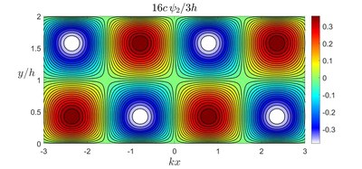
The outer steady streaming incompressible motion will depend on the geometry of the problem. If there are two walls one at [math]\displaystyle{ y=0 }[/math] and [math]\displaystyle{ y=2h }[/math], then the solution is
- [math]\displaystyle{ \psi_2 = \frac{3}{16 c}\sin 2kx\, [-(y-h) + (y-h)^3/h^2] }[/math]
which corresponds a periodic array of counter-rotating vortices, as shown in the figure.
Origin: a body force due to acoustic absorption in the fluid
Acoustic streaming is a non-linear effect. [7] We can decompose the velocity field in a vibration part and a steady part [math]\displaystyle{ {u}=v+\overline{u} }[/math]. The vibration part [math]\displaystyle{ v }[/math] is due to sound, while the steady part is the acoustic streaming velocity (average velocity). The Navier–Stokes equations implies for the acoustic streaming velocity:
- [math]\displaystyle{ \overline{\rho}{\partial_{t} \overline{u}_i}+\overline{\rho} \overline{u}_j {\partial_{j} \overline{u}_i}=-{\partial \overline{p}_{i}}+\eta {\partial^2_{j} \overline{u}_i}-{\partial_j}(\overline{\rho v_i v_j}/{\partial x_j} ). }[/math]
The steady streaming originates from a steady body force [math]\displaystyle{ f_i=-{\partial}(\overline{\rho v_i v_j} )/{\partial x_j} }[/math] that appears on the right hand side. This force is a function of what is known as the Reynolds stresses in turbulence [math]\displaystyle{ -\overline{\rho v_i v_j} }[/math]. The Reynolds stress depends on the amplitude of sound vibrations, and the body force reflects diminutions in this sound amplitude.
We see that this stress is non-linear (quadratic) in the velocity amplitude. It is non-vanishing only where the velocity amplitude varies. If the velocity of the fluid oscillates because of sound as [math]\displaystyle{ \epsilon\cos(\omega t) }[/math], the quadratic non-linearity generates a steady force proportional to [math]\displaystyle{ \scriptstyle \overline{\epsilon^2\cos^2(\omega t)}=\epsilon^2/2 }[/math].
Order of magnitude of acoustic streaming velocities
Even if viscosity is responsible for acoustic streaming, the value of viscosity disappears from the resulting streaming velocities in the case of near-boundary acoustic steaming.
The order of magnitude of streaming velocities are:[8]
- near a boundary (outside of the boundary layer):
- [math]\displaystyle{ U \sim -{3}/{(4\omega)} \times v_0 dv_0/dx, }[/math]
with [math]\displaystyle{ v_0 }[/math] the sound vibration velocity and [math]\displaystyle{ x }[/math] along the wall boundary. The flow is directed towards decreasing sound vibrations (vibration nodes).
- near a vibrating bubble[9] of rest radius a, whose radius pulsates with relative amplitude [math]\displaystyle{ \epsilon=\delta r/a }[/math] (or [math]\displaystyle{ r=\epsilon a \sin( \omega t) }[/math]), and whose center of mass also periodically translates with relative amplitude [math]\displaystyle{ \epsilon'=\delta x/a }[/math] (or [math]\displaystyle{ x=\epsilon' a \sin( \omega t/\phi) }[/math]). with a phase shift [math]\displaystyle{ \phi }[/math]
- [math]\displaystyle{ \displaystyle U \sim \epsilon \epsilon' a \omega \sin \phi }[/math]
- far from walls[10] [math]\displaystyle{ U \sim \alpha P/(\pi \mu c) }[/math] far from the origin of the flow ( with [math]\displaystyle{ P }[/math]the acoustic power, [math]\displaystyle{ \mu }[/math] the dynamic viscosity and [math]\displaystyle{ c }[/math] the celerity of sound). Nearer from the origin of the flow, the velocity scales as the root of [math]\displaystyle{ P }[/math].
- it has been shown that even biological species, e.g., adherent cells, can also exhibit acoustic streaming flow when exposed to acoustic waves. Cells adhered to a surface can generate acoustic streaming flow in the order of mm/s without being detached from the surface.[11]
See also
References
- ↑ Rayleigh, L. (1884). On the circulation of air observed in Kundt's tubes, and on some allied acoustical problems. Philosophical Transactions of the Royal Society of London, 175, 1-21.
- ↑ see video on http://lmfa.ec-lyon.fr/spip.php?article565&lang=en
- ↑ Wan, Qun; Wu, Tao; Chastain, John; Roberts, William L.; Kuznetsov, Andrey V.; Ro, Paul I. (2005). "Forced Convective Cooling via Acoustic Streaming in a Narrow Channel Established by a Vibrating Piezoelectric Bimorph". Flow, Turbulence and Combustion 74 (2): 195–206. doi:10.1007/s10494-005-4132-4.
- ↑ Nama, N., Huang, P.H., Huang, T.J., and Costanzo, F., Investigation of acoustic streaming patterns around oscillating sharp edges, Lab on a Chip, Vol. 14, pp. 2824-2836, 2014
- ↑ Salari, A.; Appak-Baskoy, S.; Ezzo, M.; Hinz, B.; Kolios, M.C.; Tsai, S.S.H. (2019) Dancing with the Cells: Acoustic Microflows Generated by Oscillating Cells. https://doi.org/10.1002/smll.201903788
- ↑ Landau, L. D., & Lifshitz, E. M. (2000). Fluid Mechanics (Course of Theoretical Physics, Volume 6).
- ↑ Sir James Lighthill (1978) "Acoustic streaming", 61, 391, Journal of Sound and Vibration
- ↑ Squires, T. M. & Quake, S. R. (2005) Microfluidics: Fluid physics at the nanoliter scale, Review of Modern Physics, vol. 77, page 977
- ↑ Longuet-Higgins, M. S. (1998). "Viscous streaming from an oscillating spherical bubble". Proc. R. Soc. Lond. A 454 (1970): 725–742. doi:10.1098/rspa.1998.0183. Bibcode: 1998RSPSA.454..725L.
- ↑ Moudjed, B.; V. Botton; D. Henry; Hamda Ben Hadid; J.-P. Garandet (2014-09-01). "Scaling and dimensional analysis of acoustic streaming jets". Physics of Fluids 26 (9): 093602. doi:10.1063/1.4895518. ISSN 1070-6631. Bibcode: 2014PhFl...26i3602M. https://hal.archives-ouvertes.fr/hal-00923712/file/Scaling_and_dimensional_analysis_of_acoustic_streaming_jets_Accepted_in_Physics_of_Fluids_HALv3.pdf.
- ↑ Salari, A.; Appak-Baskoy, S.; Ezzo, M.; Hinz, B.; Kolios, M.C.; Tsai, S.S.H. (2019) Dancing with the Cells: Acoustic Microflows Generated by Oscillating Cells. https://doi.org/10.1002/smll.201903788
 |  |

