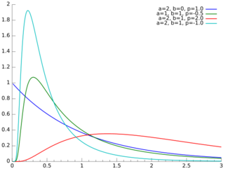
Generalized inverse Gaussian distribution

Generalized inverse Gaussian

Probability density function
Parameters	a > 0, b > 0, p real
Support	x > 0
PDF	[math]\displaystyle{ f(x) = \frac{(a/b)^{p/2}}{2 K_p(\sqrt{ab})} x^{(p-1)} e^{-(ax + b/x)/2} }[/math]
Mean	[math]\displaystyle{ \operatorname{E}[x]=\frac{\sqrt{b}\ K_{p+1}(\sqrt{a b}) }{ \sqrt{a}\ K_{p}(\sqrt{a b})} }[/math] [math]\displaystyle{ \operatorname{E}[x^{-1}]=\frac{\sqrt{a}\ K_{p+1}(\sqrt{a b}) }{ \sqrt{b}\ K_{p}(\sqrt{a b})}-\frac{2p}{b} }[/math] [math]\displaystyle{ \operatorname{E}[\ln x]=\ln \frac{\sqrt{b}}{\sqrt{a}}+\frac{\partial}{\partial p} \ln K_{p}(\sqrt{a b}) }[/math]
Mode	[math]\displaystyle{ \frac{(p-1)+\sqrt{(p-1)^2+ab}}{a} }[/math]
Variance	[math]\displaystyle{ \left(\frac{b}{a}\right)\left[\frac{K_{p+2}(\sqrt{ab})}{K_p(\sqrt{ab})}-\left(\frac{K_{p+1}(\sqrt{ab})}{K_p(\sqrt{ab})}\right)^2\right] }[/math]
MGF	[math]\displaystyle{ \left(\frac{a}{a-2t}\right)^{\frac{p}{2}}\frac{K_p(\sqrt{b(a-2t)})}{K_p(\sqrt{ab})} }[/math]
CF	[math]\displaystyle{ \left(\frac{a}{a-2it}\right)^{\frac{p}{2}}\frac{K_p(\sqrt{b(a-2it)})}{K_p(\sqrt{ab})} }[/math]

In probability theory and statistics, the generalized inverse Gaussian distribution (GIG) is a three-parameter family of continuous probability distributions with probability density function

[math]\displaystyle{ f(x) = \frac{(a/b)^{p/2}}{2 K_p(\sqrt{ab})} x^{(p-1)} e^{-(ax + b/x)/2},\qquad x\gt 0, }[/math]

where K_p is a modified Bessel function of the second kind, a > 0, b > 0 and p a real parameter. It is used extensively in geostatistics, statistical linguistics, finance, etc. This distribution was first proposed by Étienne Halphen. It was rediscovered and popularised by Ole Barndorff-Nielsen, who called it the generalized inverse Gaussian distribution. Its statistical properties are discussed in Bent Jørgensen's lecture notes.

Properties

Alternative parametrization

By setting [math]\displaystyle{ \theta = \sqrt{ab} }[/math] and [math]\displaystyle{ \eta = \sqrt{b/a} }[/math], we can alternatively express the GIG distribution as

[math]\displaystyle{ f(x) = \frac{1}{2\eta K_p(\theta)} \left(\frac{x}{\eta}\right)^{p-1} e^{-\theta(x/\eta + \eta/x)/2}, }[/math]

where [math]\displaystyle{ \theta }[/math] is the concentration parameter while [math]\displaystyle{ \eta }[/math] is the scaling parameter.

Summation

Barndorff-Nielsen and Halgreen proved that the GIG distribution is infinitely divisible.

Entropy

The entropy of the generalized inverse Gaussian distribution is given as

[math]\displaystyle{ \begin{align} H = \frac{1}{2} \log \left( \frac b a \right) & {} +\log \left(2 K_p\left(\sqrt{ab} \right)\right) - (p-1) \frac{\left[\frac{d}{d\nu}K_\nu\left(\sqrt{ab}\right)\right]_{\nu=p}}{K_p\left(\sqrt{a b}\right)} \\ & {} + \frac{\sqrt{a b}}{2 K_p\left(\sqrt{a b}\right)}\left( K_{p+1}\left(\sqrt{ab}\right) + K_{p-1}\left(\sqrt{a b}\right)\right) \end{align} }[/math]

where [math]\displaystyle{ \left[\frac{d}{d\nu}K_\nu\left(\sqrt{a b}\right)\right]_{\nu=p} }[/math] is a derivative of the modified Bessel function of the second kind with respect to the order [math]\displaystyle{ \nu }[/math] evaluated at [math]\displaystyle{ \nu=p }[/math]

Characteristic Function

The characteristic of a random variable [math]\displaystyle{ X\sim GIG(p, a, b) }[/math] is given as(for a derivation of the characteristic function, see supplementary materials of )

[math]\displaystyle{ E(e^{itX}) = \left(\frac{a }{a-2it }\right)^{\frac{p}{2}} \frac{K_{p}\left( \sqrt{(a-2it)b} \right)}{ K_{p}\left( \sqrt{ab} \right) } }[/math]

for [math]\displaystyle{ t \in \mathbb{R} }[/math] where [math]\displaystyle{ i }[/math] denotes the imaginary number.

Related distributions

Special cases

The inverse Gaussian and gamma distributions are special cases of the generalized inverse Gaussian distribution for p = −1/2 and b = 0, respectively. Specifically, an inverse Gaussian distribution of the form

[math]\displaystyle{ f(x;\mu,\lambda) = \left[\frac{\lambda}{2 \pi x^3}\right]^{1/2} \exp{ \left( \frac{-\lambda (x-\mu)^2}{2 \mu^2 x} \right)} }[/math]

is a GIG with [math]\displaystyle{ a = \lambda/\mu^2 }[/math], [math]\displaystyle{ b = \lambda }[/math], and [math]\displaystyle{ p=-1/2 }[/math]. A Gamma distribution of the form

[math]\displaystyle{ g(x;\alpha,\beta) = \beta^\alpha \frac 1 {\Gamma(\alpha)} x^{\alpha-1} e^{-\beta x} }[/math]

is a GIG with [math]\displaystyle{ a = 2 \beta }[/math], [math]\displaystyle{ b = 0 }[/math], and [math]\displaystyle{ p = \alpha }[/math].

Other special cases include the inverse-gamma distribution, for a = 0.

Conjugate prior for Gaussian

The GIG distribution is conjugate to the normal distribution when serving as the mixing distribution in a normal variance-mean mixture. Let the prior distribution for some hidden variable, say [math]\displaystyle{ z }[/math], be GIG:

[math]\displaystyle{ P(z\mid a,b,p) = \operatorname{GIG}(z\mid a,b,p) }[/math]

and let there be [math]\displaystyle{ T }[/math] observed data points, [math]\displaystyle{ X=x_1,\ldots,x_T }[/math], with normal likelihood function, conditioned on [math]\displaystyle{ z: }[/math]

[math]\displaystyle{ P(X\mid z,\alpha,\beta) = \prod_{i=1}^T N(x_i\mid\alpha+\beta z,z) }[/math]

where [math]\displaystyle{ N(x\mid\mu,v) }[/math] is the normal distribution, with mean [math]\displaystyle{ \mu }[/math] and variance [math]\displaystyle{ v }[/math]. Then the posterior for [math]\displaystyle{ z }[/math], given the data is also GIG:

[math]\displaystyle{ P(z\mid X,a,b,p,\alpha,\beta) = \text{GIG}\left(z\mid a+T\beta^2,b+S,p-\frac T 2 \right) }[/math]

where [math]\displaystyle{ \textstyle S = \sum_{i=1}^T (x_i-\alpha)^2 }[/math].

Sichel distribution

The Sichel distribution results when the GIG is used as the mixing distribution for the Poisson parameter [math]\displaystyle{ \lambda }[/math].

See also

• Inverse Gaussian distribution
• Gamma distribution

References

- ↑ Seshadri, V. (1997). "Halphen's laws". in Kotz, S.; Read, C. B.; Banks, D. L.. Encyclopedia of Statistical Sciences, Update Volume 1. New York: Wiley. pp. 302–306.
- ↑ Perreault, L.; Bobée, B.; Rasmussen, P. F. (1999). "Halphen Distribution System. I: Mathematical and Statistical Properties". Journal of Hydrologic Engineering 4 (3): 189. doi:10.1061/(ASCE)1084-0699(1999)4:3(189).
- ↑ Étienne Halphen was the grandson of the mathematician Georges Henri Halphen.
- ↑ Jørgensen, Bent (1982). Statistical Properties of the Generalized Inverse Gaussian Distribution. Lecture Notes in Statistics. 9. New York–Berlin: Springer-Verlag. ISBN 0-387-90665-7.
- ↑ O. Barndorff-Nielsen and Christian Halgreen, Infinite Divisibility of the Hyperbolic and Generalized Inverse Gaussian Distributions, Zeitschrift für Wahrscheinlichkeitstheorie und verwandte Gebiete 1977
- ↑ Pal, Subhadip; Gaskins, Jeremy (23 May 2022). "Modified Pólya-Gamma data augmentation for Bayesian analysis of directional data". Journal of Statistical Computation and Simulation 92 (16): 3430–3451. doi:10.1080/00949655.2022.2067853. ISSN 0094-9655. https://www.tandfonline.com/doi/abs/10.1080/00949655.2022.2067853?journalCode=gscs20.
- ↑ 7.0 7.1 Johnson, Norman L.; Kotz, Samuel; Balakrishnan, N. (1994), Continuous univariate distributions. Vol. 1, Wiley Series in Probability and Mathematical Statistics: Applied Probability and Statistics (2nd ed.), New York: John Wiley & Sons, pp. 284–285, ISBN 978-0-471-58495-7
- ↑ Dimitris Karlis, "An EM type algorithm for maximum likelihood estimation of the normal–inverse Gaussian distribution", Statistics & Probability Letters 57 (2002) 43–52.
- ↑ Barndorf-Nielsen, O.E., 1997. Normal Inverse Gaussian Distributions and stochastic volatility modelling. Scand. J. Statist. 24, 1–13.
- ↑ Sichel, Herbert S, 1975. "On a distribution law for word frequencies." Journal of the American Statistical Association 70.351a: 542-547.
- ↑ Stein, Gillian Z., Walter Zucchini, and June M. Juritz, 1987. "Parameter estimation for the Sichel distribution and its multivariate extension." Journal of the American Statistical Association 82.399: 938-944.