Folding (DSP implementation)
Folding [1] is a transformation technique using in DSP architecture implementation for minimizing the number of functional blocks in synthesizing DSP architecture. Folding was first developed by Keshab K. Parhi and his students in 1992. Its concept is contrary to unfolding. Folding transforms an operation from a unit-time processing to N unit-times processing where N is called folding factor. Therefore, multiple same operations (less than N) used in original system could be replaced with a signal operation block in transformed system. Thus, in N unit-times, a functional block in transformed system could be reused to perform N operations in original system.
While the folding transformation reduces the number of functional units in the architecture, it needs more memory element to store the temporary data. The reason is that multiple data produced from an operation block needs to be distinguished from N data produced from original operations. Therefore, the number of register may be increased. Furthermore, it needs additional multiplexer for switching different operation paths. Hence, the number of switching elements would also be increased. To counterattack such issues, the considerations of folding is
- How to schedule multiple operations into an operation block.
- How to schedule the memory element for reducing the number of registers and multiplexers.
Example
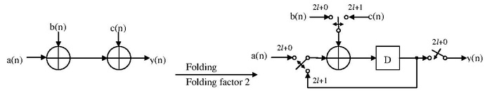
The following graph shows the example of folding transformation. The original DSP system produces y(n) at each unit time. The transformed DSP system produces y(n) in each 2 l where each 2 l increase 1 n, index of y. The resource used in original system are 2 adders, and the resource used in transformed system are 1 adder, 1 register, 3 multiplexer. The functional block, adder, is therefore reduced.
Algorithm
The DSP implementation in the folding algorithm is a Data flow graph(DFG), which is a graph composed of functional nodes and delay edges.
Another input for folding algorithm is folding set which is the function maps an operation unit of original DFG to an operation of transformed DFG with the number n <= N indicated the order of reused operation.
Given a DFG, a folding factor N, and folding set. The transformation is performing:
- Creating folded nodes which are the node of the image of folding set.
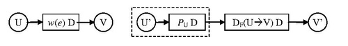
- Computing the delay elements for storing the distinguished data among different operation cycles as equation:
- [math]\displaystyle{ D_F(U\xrightarrow{e}V)=Nw(e)-P_U+v-u }[/math] where
- [math]\displaystyle{ \scriptstyle D_F }[/math] is the number of delay elements needed between element [math]\displaystyle{ \scriptstyle U,V }[/math], the operation units of original DFG.
- [math]\displaystyle{ \scriptstyle w(e) }[/math] is the delay elements used in original DFG between [math]\displaystyle{ \scriptstyle U,V }[/math].
- [math]\displaystyle{ \scriptstyle u }[/math] is the order of [math]\displaystyle{ \scriptstyle U }[/math] in the transformed operation block.
- [math]\displaystyle{ \scriptstyle v }[/math] is the order of [math]\displaystyle{ \scriptstyle V }[/math] in the transformed operation block.
- [math]\displaystyle{ \scriptstyle P_U }[/math] is the internal delay in transformed operation of [math]\displaystyle{ \scriptstyle U }[/math].
- Merging the delay elements forms the data path between the functional elements in transformed DFG.
Biquad filter example
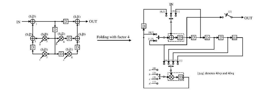
The following graph show the example of folding algorithm. The folding set is [math]\displaystyle{ \scriptstyle \{S_i|j\} }[/math] where [math]\displaystyle{ \scriptstyle S_i }[/math] is the transformed operator and [math]\displaystyle{ \scriptstyle j }[/math] is the order of such operator. Therefore, the image of the folding set are [math]\displaystyle{ \scriptstyle S_1,S_2 }[/math] representing adder and multiplier respectively. Furthermore, in this example, we use the pipelining adder and multiplier which have 1 and 2 delay respectively in right graph.
Next, we compute the delay elements for storing the data.
- [math]\displaystyle{ \scriptstyle D_F(1\rightarrow 2)= 4(1)-1+1-3=1 }[/math]
- [math]\displaystyle{ \scriptstyle D_F(1\rightarrow 5)= 4(1)-1+0-3=0 }[/math]
- [math]\displaystyle{ \scriptstyle D_F(1\rightarrow 6)= 4(1)-1+2-3=2 }[/math]
- [math]\displaystyle{ \scriptstyle D_F(1\rightarrow 7)= 4(1)-1+3-3=3 }[/math]
- [math]\displaystyle{ \scriptstyle D_F(1\rightarrow 8)= 4(2)-1+1-3=5 }[/math]
- [math]\displaystyle{ \scriptstyle D_F(3\rightarrow 1)= 4(0)-1+3-2=0 }[/math]
- [math]\displaystyle{ \scriptstyle D_F(4\rightarrow 2)= 4(0)-1+1-0=0 }[/math]
- [math]\displaystyle{ \scriptstyle D_F(5\rightarrow 3)= 4(0)-2+2-0=0 }[/math]
- [math]\displaystyle{ \scriptstyle D_F(6\rightarrow 4)= 4(1)-2+0-2=0 }[/math]
- [math]\displaystyle{ \scriptstyle D_F(7\rightarrow 3)= 4(1)-2+2-3=1 }[/math]
- [math]\displaystyle{ \scriptstyle D_F(8\rightarrow 4)= 4(1)-2+0-1=1 }[/math]
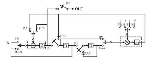
After computing the delay element needed, we construct the data path to connect the functional blocks with corresponding multiplexer. The final graph is shown as below where [math]\displaystyle{ \scriptstyle \{i,j\} }[/math] represents the switching moment.
Register minimization
[2] In the above example, if we perform register minimization, we could reduce the number of register significantly. The technique for minimizing register is call lifetime analysis, which analyzes the time for when a data is produced and when a data finally s consumed. The time for producing a data is denoted [math]\displaystyle{ \scriptstyle T_{input} }[/math], and the time for the last consumed data is denoted [math]\displaystyle{ \scriptstyle T_{output} }[/math].
- [math]\displaystyle{ \scriptstyle T_{input}=u+P_U }[/math] where u is the folding order of [math]\displaystyle{ \scriptstyle U }[/math] and [math]\displaystyle{ \scriptstyle P_U }[/math] is the number of pipelining stages in the functional unit that executes [math]\displaystyle{ \scriptstyle u }[/math].
- [math]\displaystyle{ \scriptstyle T_{output} }[/math] for the node [math]\displaystyle{ \scriptstyle U }[/math] is [math]\displaystyle{ \scriptstyle u+P_U+max_V\{D_F(U\rightarrow V)\} }[/math]
Therefore, we could perform life time analysis from the above example as following table.
| node | [math]\displaystyle{ \scriptstyle T_{input} }[/math] | [math]\displaystyle{ \scriptstyle T_{output} }[/math] |
|---|---|---|
| 1 | 4 | 9 |
| 2 | 2 | 2 |
| 3 | 3 | 3 |
| 4 | 1 | 1 |
| 5 | 2 | 2 |
| 6 | 4 | 4 |
| 7 | 5 | 6 |
| 8 | 3 | 4 |
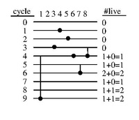
From the life time analyzing above, we could analyze the minimal register needed. In this case, we construct the lifetime chart corresponding to the lifetime table in above. For node 1, we plot a horizontal line from cycle 4 to 9 indicating that the data is need to be stored from cycle 4 to cycle 9. In the same method, we could construct the chart to indicating that how many data need to be stored in each cycle. Hence, cycle 6 needs to store 2 data. Maximum number of data need to be store d in this example is 2. Hence, we allocate 2 delay element for constructing the transformed data path.
After allocating 2 delay element for storing the temporary data, we need to schedule data stored at which register. The following table shows the data stored in each register R1 and R2, such that the number of multiplexer could be minimized.
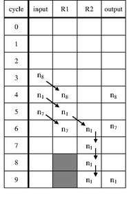
Finally, we could reconstruct the data path with fewer delay element and switching element in the folded design.
See also
References
- ↑ K. K. Parhi, C.-Y. Wang, and A. P. Brown, "synthesis of control circuits in folded pipelined DSP architectures," IEEE Journal of Solid-State Circuits, vol. 27, no. 1, pp. 29-43, Jan. 1992
- ↑ K.K. Parhi, "Systematic synthesis of DSP data format converters using life time analysis and forward-backward register allocation," IEEE Trans. on Circuits and Systems -II, vol. 39, no. 7, pp.423-440, July 1992
 |  |

