Delta set
In mathematics, a Δ-set S, often called a Δ-complex or a semi-simplicial set, is a combinatorial object that is useful in the construction and triangulation of topological spaces, and also in the computation of related algebraic invariants of such spaces. A Δ-set is somewhat more general than a simplicial complex, yet not quite as sophisticated as a simplicial set. Simplicial sets have additional structure, so that every simplicial set is also a semi-simplicial set.

As an example, suppose we want to triangulate the 1-dimensional circle [math]\displaystyle{ S^1 }[/math]. To do so with a simplicial complex, we need at least three vertices, and edges connecting them. But delta-sets allow for a simpler triangulation: thinking of [math]\displaystyle{ S^1 }[/math] as the interval [0,1] with the two endpoints identified, we can define a triangulation with a single vertex 0, and a single edge looping between 0 and 0.
Formally, a Δ-set is a sequence of sets [math]\displaystyle{ \{S_n\}_{n=0}^{\infty} }[/math] together with maps
- [math]\displaystyle{ d_i^n \colon S_{n+1} \rightarrow S_n }[/math]
for each [math]\displaystyle{ n\geq 0 }[/math] and [math]\displaystyle{ i=0,1,\dots,n+1 }[/math], that satisfy
- [math]\displaystyle{ d_i^{n}\circ d_j^{n+1}=d_{j-1}^{n}\circ d_i^{n+1} }[/math]
whenever [math]\displaystyle{ i \lt j }[/math]. Often, the superscript of [math]\displaystyle{ {d_i^n} }[/math] is omitted for brevity.
This definition generalizes the notion of a simplicial complex, where the [math]\displaystyle{ S_n }[/math] are the sets of n-simplices, and the [math]\displaystyle{ d_i }[/math] are the associated face maps, each mapping the [math]\displaystyle{ i }[/math]-th face of a simplex in [math]\displaystyle{ S_{n+1} }[/math] to a simplex in [math]\displaystyle{ S_{n} }[/math]. The composition rule ensures that the faces in [math]\displaystyle{ S_{n+1} }[/math] of a simplex in [math]\displaystyle{ S_{n+2} }[/math] share their neighboring faces in [math]\displaystyle{ S_n }[/math], i.e. that the simplexes are well-formed. Δ-set is not as general as a simplicial set, since it lacks "degeneracies".

Given Δ-sets S and T, a map of Δ-sets is a collection of set-maps
- [math]\displaystyle{ \{ f_n\colon S_n \rightarrow T_n \}_{n=0}^{\infty} }[/math]
such that
- [math]\displaystyle{ f_n \circ d_i = d_i \circ f_{n+1} }[/math]
whenever both sides of the equation are defined.
With this notion, we can define the category of Δ-sets, whose objects are Δ-sets and whose morphisms are maps of Δ-sets.
Each Δ-set has a corresponding geometric realization, associating a geometrically defined space (a standard n-simplex) with each abstract simplex in Δ-set, and then "gluing" the spaces together using inclusion relations between the spaces to define an equivalence relation:
- [math]\displaystyle{ |S| = \left( \coprod_{n=0}^{\infty} S_n \times \Delta^n \right)/_{\sim} }[/math]
where we declare [math]\displaystyle{ {\sim} }[/math] as
- [math]\displaystyle{ (\sigma,\iota ^i t) \sim (d_i \sigma, t) \quad \text{ for all } \sigma \in S_n, t \in \Delta^{n-1}. }[/math]
Here, [math]\displaystyle{ \Delta^n }[/math] denotes a standard n-simplex as a space, and
- [math]\displaystyle{ \iota^i \colon \Delta^{n-1} \rightarrow \Delta^n }[/math]
is the inclusion of the i-th face. The geometric realization is a topological space with the quotient topology.
The geometric realization of a Δ-set S has a natural filtration
- [math]\displaystyle{ |S|_0 \subset |S|_1 \subset \cdots \subset |S|, }[/math]
where
- [math]\displaystyle{ |S|_N = \left( \coprod_{n=0}^{N} S_n \times \Delta^n \right)/_{\sim} }[/math]
is a "restricted" geometric realization.
Related functors
The geometric realization of a Δ-set described above defines a covariant functor from the category of Δ-sets to the category of topological spaces. Geometric realization takes a Δ-set to a topological space, and carries maps of Δ-sets to induced continuous maps between geometric realizations.
If S is a Δ-set, there is an associated free abelian chain complex, denoted [math]\displaystyle{ (\Z S, \partial ) }[/math], whose n-th group is the free abelian group
- [math]\displaystyle{ (\Z S)_n = \Z \langle S_n \rangle, }[/math]
generated by the set [math]\displaystyle{ S_n }[/math], and whose n-th differential is defined by
- [math]\displaystyle{ \partial_n = d_0 - d_1 + d_2 - \cdots + (-1)^n d_n. }[/math]
This defines a covariant functor from the category of Δ-sets to the category of chain complexes of abelian groups. A Δ-set is carried to the chain complex just described, and a map of Δ-sets is carried to a map of chain complexes, which is defined by extending the map of Δ-sets in the standard way using the universal property of free abelian groups.
Given any topological space X, one can construct a Δ-set [math]\displaystyle{ \mathrm{sing}(X) }[/math] as follows. A singular n-simplex in X is a continuous map
- [math]\displaystyle{ \sigma \colon \Delta^n \rightarrow X. }[/math]
Define
- [math]\displaystyle{ \mathrm{sing}_n^{}(X) }[/math]
to be the collection of all singular n-simplicies in X, and define
- [math]\displaystyle{ d_i \colon \mathrm{sing}_{i+1}(X) \rightarrow \mathrm{sing}_i(X) }[/math]
by
- [math]\displaystyle{ d_i(\sigma) = \sigma \circ d^i, }[/math]
where again [math]\displaystyle{ d^i }[/math] is the [math]\displaystyle{ i }[/math]-th face map. One can check that this is in fact a Δ-set. This defines a covariant functor from the category of topological spaces to the category of Δ-sets. A topological space is carried to the Δ-set just described, and a continuous map of spaces is carried to a map of Δ-sets, which is given by composing the map with the singular n-simplices.
Examples
This example illustrates the constructions described above. We can create a Δ-set S whose geometric realization is the unit circle [math]\displaystyle{ S^1 }[/math], and use it to compute the homology of this space. Thinking of [math]\displaystyle{ S^1 }[/math] as an interval with the endpoints identified, define
- [math]\displaystyle{ S_0 = \{v\}, \quad S_1 = \{e\}, }[/math]
with [math]\displaystyle{ S_n = \varnothing }[/math] for all [math]\displaystyle{ n \ge 2 }[/math]. The only possible maps [math]\displaystyle{ d_0,d_1\colon S_1 \rightarrow S_0, }[/math] are
- [math]\displaystyle{ d_0(e) = d_1(e) = v. \quad }[/math]
It is simple to check that this is a Δ-set, and that [math]\displaystyle{ |S| \cong S^1 }[/math]. Now, the associated chain complex [math]\displaystyle{ (\Z S,\partial) }[/math] is
- [math]\displaystyle{ 0 \longrightarrow \Z \langle e \rangle \stackrel{\partial_1}{\longrightarrow} \Z \langle v \rangle \longrightarrow 0, }[/math]
where
- [math]\displaystyle{ \partial_1(e) = d_0(e) - d_1(e) = v - v = 0. }[/math]
In fact, [math]\displaystyle{ \partial_n = 0 }[/math] for all n. The homology of this chain complex is also simple to compute:
- [math]\displaystyle{ H_0(\Z S) = \frac{\ker \partial_0}{\mathrm{im} \partial_1} = \mathbb{Z} \langle v \rangle \cong \Z, }[/math]
- [math]\displaystyle{ H_1(\Z S) = \frac{\ker \partial_1}{\mathrm{im} \partial_2} = \mathbb{Z} \langle e \rangle \cong \Z. }[/math]
All other homology groups are clearly trivial.
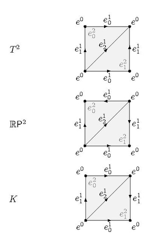
The following example is from section 2.1 of Hatcher's Algebraic Topology.[1] Consider the Δ-set structure given to the torus in the figure, which has one vertex, three edges, and two 2-simplices.
The boundary map [math]\displaystyle{ \partial_1 }[/math] is 0 because there is only one vertex, so [math]\displaystyle{ H_0(T^2) = \text{ker } \partial_0/\text{ im } \partial_1 = \mathbb{Z} }[/math]. Let [math]\displaystyle{ \{e_0^1, e_1^1,e_0^1+e_1^1-e_2^1\} }[/math] be a basis for [math]\displaystyle{ \Delta_1(T^2) }[/math]. Then [math]\displaystyle{ \partial_2(e_0^2) = e_0^1+e_1^1-e_2^1= \partial_2(e_1^2) }[/math], so [math]\displaystyle{ \text{im } \partial_2 = \langle e_0^1+e_1^1-e_2^1 \rangle }[/math], and hence [math]\displaystyle{ H_1(T^2) = \text{ker }\partial_1 / \text{ im } \partial_2 = \mathbb{Z}^3/\mathbb{Z} = \mathbb{Z}^2. }[/math]
Since there are no 3-simplices, [math]\displaystyle{ H_2(T^2)=\text{ker } \partial_2 }[/math]. We have that [math]\displaystyle{ \partial_2(p e_0^2 + q e_1^2) = (p+q) (e_0^1+e_1^1-e_2^1) }[/math] which is 0 if and only if [math]\displaystyle{ p=-q }[/math]. Hence [math]\displaystyle{ \text{ker } \partial_2 }[/math] is infinite cyclic generated by [math]\displaystyle{ e_0^2-e_1^2 }[/math].
So [math]\displaystyle{ H_2(T^2)=\mathbb{Z} }[/math]. Clearly [math]\displaystyle{ H_n(T^2)=0 }[/math] for [math]\displaystyle{ n\ge 3. }[/math]
Thus, [math]\displaystyle{ H_n(T^2) = \begin{cases} \mathbb{Z} & n=0,2\\ \mathbb{Z}^2 & n=1\\ 0 & n\ge 3. \end{cases} }[/math]
It is worth highlighting that the minimum number of simplices needed to endow [math]\displaystyle{ T^2 }[/math] with the structure of a simplicial complex is 7 vertices, 21 edges, and 14 2-simplices, for a total of 42 simplices. This would make the above calculations, which only used 6 simplices, much harder for someone to do by hand.
This is a non-example. Consider a line segment. This is a 1-dimensional Δ-set and a 1-dimensional simplicial set. However, if we view the line segment as a 2-dimensional simplicial set, in which the 2-simplex is viewed as degenerate, then the line segment is not a Δ-set, as we do not allow for such degeneracies.
Abstract nonsense
We now inspect the relation between Δ-sets and simplicial sets. Consider the simplex category [math]\displaystyle{ \Delta }[/math], whose objects are the finite totally ordered sets [math]\displaystyle{ [n] := \{0, 1,\cdots , n\} }[/math] and whose morphisms are monotone maps. A simplicial set is defined to be a presheaf on [math]\displaystyle{ \Delta }[/math], i.e. a (contravariant) functor [math]\displaystyle{ S: \Delta^{\text{op}} \to \text{Set} }[/math]. On the other hand, consider the subcategory [math]\displaystyle{ \hat{\Delta} }[/math] of [math]\displaystyle{ \Delta }[/math] whose morphisms are only the strict monotone maps. Note that the morphisms in [math]\displaystyle{ \hat{\Delta} }[/math] are precisely the injections in [math]\displaystyle{ \Delta }[/math], and one can prove that these are generated by the monotone maps of the form [math]\displaystyle{ \delta^i: [n] \to [n+1] }[/math] which "skip" the element [math]\displaystyle{ i \in [n+1] }[/math]. From this we see that a presheaf [math]\displaystyle{ S: \hat{\Delta}^{\text{op}} \to \text{Set} }[/math] on [math]\displaystyle{ \hat{\Delta} }[/math] is determined by a sequence of sets [math]\displaystyle{ \{S_n\}_{n = 0}^\infty }[/math] (where we denote [math]\displaystyle{ S([n]) }[/math] by [math]\displaystyle{ S_n }[/math] for simplicity) together with maps [math]\displaystyle{ d_i: S_{n+1} \to S_{n} }[/math] for [math]\displaystyle{ i = 0,1,\ldots,n+1 }[/math] (where we denote [math]\displaystyle{ S(\delta^i) }[/math] by [math]\displaystyle{ d_i }[/math] for simplicity as well). In fact, after checking that [math]\displaystyle{ \delta^j \circ \delta^i = \delta^i \circ \delta^{j-1} }[/math] in [math]\displaystyle{ \hat{\Delta} }[/math], one concludes that
- [math]\displaystyle{ d_i \circ d_j = d_{j-1} \circ d_i }[/math]
whenever [math]\displaystyle{ i \lt j }[/math]. Thus, a presheaf on [math]\displaystyle{ \hat{\Delta} }[/math] determines the data of a Δ-set and, conversely, all Δ-sets arise in this way.[2] Moreover, Δ-maps [math]\displaystyle{ f: S \to T }[/math] between Δ-sets correspond to natural transformations when we view [math]\displaystyle{ S }[/math] and [math]\displaystyle{ T }[/math] as (contravariant) functors. In this sense, Δ-sets are presheaves on [math]\displaystyle{ \hat{\Delta} }[/math] while simplicial sets are presheaves on [math]\displaystyle{ \Delta }[/math].
From this perspective, it is now easy to see that every simplicial set is a Δ-set. Indeed, notice there is an inclusion [math]\displaystyle{ \hat{\Delta} \hookrightarrow \Delta }[/math]; so that every simplicial set [math]\displaystyle{ S: \Delta^{\text{op}} \to \text{Set} }[/math] naturally gives rise to a Δ-set, namely the composite [math]\displaystyle{ \hat{\Delta}^{\text{op}} \hookrightarrow \Delta^{\text{op}} \xrightarrow{S} \text{Set} }[/math].
Pros and cons
One advantage of using Δ-sets in this way is that the resulting chain complex is generally much simpler than the singular chain complex. For reasonably simple spaces, all of the groups will be finitely generated, whereas the singular chain groups are, in general, not even countably generated.
One drawback of this method is that one must prove that the geometric realization of the Δ-set is actually homeomorphic to the topological space in question. This can become a computational challenge as the Δ-set increases in complexity.
See also
References
- ↑ Hatcher, Allen (2002). Algebraic topology. Cambridge: Cambridge University Press. ISBN 0-521-79160-X. OCLC 45420394. https://www.worldcat.org/oclc/45420394.
- ↑ Friedman, Greg (2012). "Survey article: An elementary illustrated introduction to simplicial sets". The Rocky Mountain Journal of Mathematics 42 (2): 353–423. doi:10.1216/RMJ-2012-42-2-353.
- Ranicki, Andrew A. (1993). Algebraic L-theory and Topological Manifolds. Cambridge Tracts in Mathematics. 102. Cambridge Univ. Press. ISBN 978-0-521-42024-2. http://www.maths.ed.ac.uk/~aar/books/topman.pdf.
- "On The Algebraic L-theory of Δ-sets". Pure and Applied Mathematics Quarterly 8 (2): 423–450. 2012. doi:10.4310/pamq.2012.v8.n2.a3.
- Rourke, Colin P.; Sanderson, Brian J. (1971). "Δ-Sets I: Homotopy Theory". Quarterly Journal of Mathematics 22 (3): 321–338. doi:10.1093/qmath/22.3.321. Bibcode: 1971QJMat..22..321R.
 |  |

