Blancmange curve

In mathematics, the blancmange curve is a self-affine curve constructible by midpoint subdivision. It is also known as the Takagi curve, after Teiji Takagi who described it in 1901, or as the Takagi–Landsberg curve, a generalization of the curve named after Takagi and Georg Landsberg. The name blancmange comes from its resemblance to a Blancmange pudding. It is a special case of the more general de Rham curve; see also fractal curve.
Definition
The blancmange function is defined on the unit interval by
- [math]\displaystyle{ {\rm blanc}(x) = \sum_{n=0}^\infty {s(2^{n}x)\over 2^n}, }[/math]
where [math]\displaystyle{ s(x) }[/math] is the triangle wave, defined by [math]\displaystyle{ s(x)=\min_{n\in{\mathbf Z}}|x-n| }[/math], that is, [math]\displaystyle{ s(x) }[/math] is the distance from x to the nearest integer.
The Takagi–Landsberg curve is a slight generalization, given by
- [math]\displaystyle{ T_w(x) = \sum_{n=0}^\infty w^n s(2^{n}x) }[/math]
for a parameter [math]\displaystyle{ w }[/math]; thus the blancmange curve is the case [math]\displaystyle{ w=1/2 }[/math]. The value [math]\displaystyle{ H=-\log_2 w }[/math] is known as the Hurst parameter.
The function can be extended to all of the real line: applying the definition given above shows that the function repeats on each unit interval.
The function could also be defined by the series in the section Fourier series expansion.
Functional equation definition
The periodic version of the Takagi curve can also be defined as the unique bounded solution [math]\displaystyle{ T=T_w:\R\to\R }[/math] to the functional equation
- [math]\displaystyle{ T(x) = s(x) + w T(2x) }[/math].
Indeed, the blancmange function [math]\displaystyle{ T_w }[/math] is certainly bounded, and solves the functional equation, since
- [math]\displaystyle{ T_w(x) := \sum_{n=0}^\infty w^n s(2^{n}x)= s(x) + \sum_{n=1}^\infty w^n s(2^{n}x) }[/math][math]\displaystyle{ = s(x) + w\sum_{n=0}^\infty w^n s(2^{n+1}x)= s(x) + wT_w(2x) }[/math].
Conversely, if [math]\displaystyle{ T:\R\to\R }[/math] is a bounded solution of the functional equation, iterating the equality one has for any N
- [math]\displaystyle{ T(x) =\sum_{n=0}^N w^n s(2^{n}x) + w^{N+1} T(2^{N+1}x) =\sum_{n=0}^N w^n s(2^{n}x) + o(1) }[/math], for [math]\displaystyle{ N\to\infty, }[/math]
whence [math]\displaystyle{ T=T_w }[/math]. Incidentally, the above functional equations possesses infinitely many continuous, non-bounded solutions, e.g. [math]\displaystyle{ T_w(x)+ c |x|^{-\log_2 w }. }[/math]
Graphical construction
The blancmange curve can be visually built up out of triangle wave functions if the infinite sum is approximated by finite sums of the first few terms. In the illustrations below, progressively finer triangle functions (shown in red) are added to the curve at each stage.
 |
192px | 192px | 
|
| n = 0 | n ≤ 1 | n ≤ 2 | n ≤ 3 |
Properties
Convergence and continuity
The infinite sum defining [math]\displaystyle{ T_w(x) }[/math] converges absolutely for all [math]\displaystyle{ x }[/math]: since [math]\displaystyle{ 0\le s(x) \le 1/2 }[/math] for all [math]\displaystyle{ x\in \mathbb{R} }[/math], we have:
- [math]\displaystyle{ \sum_{n=0}^\infty |w^n s(2^n x)| \le \frac{1}{2} \sum_{n=0}^\infty |w|^n = \frac{1}{2} \cdot \frac{1}{1-|w|} }[/math] if [math]\displaystyle{ |w|\lt 1 }[/math].
Therefore, the Takagi curve of parameter [math]\displaystyle{ w }[/math] is defined on the unit interval (or [math]\displaystyle{ \mathbb{R} }[/math]) if [math]\displaystyle{ |w|\lt 1 }[/math].
The Takagi function of parameter [math]\displaystyle{ w }[/math] is continuous. Indeed, the functions [math]\displaystyle{ T_{w,n} }[/math] defined by the partial sums [math]\displaystyle{ T_{w,n}(x) = \sum_{k=0}^n w^k s(2^k x) }[/math] are continuous and converge uniformly toward [math]\displaystyle{ T_w }[/math], since:
- [math]\displaystyle{ \left|T_w(x) - T_{w,n}(x)\right| = \left|\sum_{k=n+1}^\infty w^k s(2^k x)\right| = \left|w^{n+1} \sum_{k=0}^\infty w^k s(2^{k+n+1} x)\right| \le \frac{|w|^{n+1}}{2} \cdot \frac{1}{1-|w|} }[/math] for all x when [math]\displaystyle{ |w| \lt 1 }[/math].
This value can be made as small as we want by selecting a big enough value of n. Therefore, by the uniform limit theorem, [math]\displaystyle{ T_w }[/math] is continuous if |w|<1.
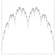
parameter w=2/3
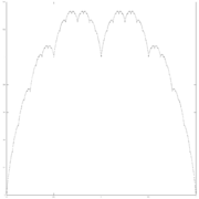
parameter w=1/2
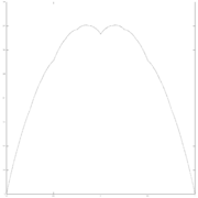
parameter w=1/3
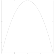
parameter w=1/4
parameter w=1/8


Subadditivity
Since the absolute value is a subadditive function so is the function [math]\displaystyle{ s(x)=\min_{n\in{\mathbf Z}}|x-n| }[/math], and its dilations [math]\displaystyle{ s(2^kx) }[/math]; since positive linear combinations and point-wise limits of subadditive functions are subadditive, the Takagi function is subadditive for any value of the parameter [math]\displaystyle{ w }[/math].
The special case of the parabola
For [math]\displaystyle{ w=1/4 }[/math], one obtains the parabola: the construction of the parabola by midpoint subdivision was described by Archimedes.
Differentiability
For values of the parameter [math]\displaystyle{ 0\lt w \lt 1/2 }[/math] the Takagi function [math]\displaystyle{ T_w }[/math] is differentiable in classical sense at any [math]\displaystyle{ x\in\R }[/math] which is not a dyadic rational. Precisely, by derivation under the sign of series, for any non dyadic rational [math]\displaystyle{ x\in\R }[/math] one finds
- [math]\displaystyle{ T_w'(x) = \sum_{n=0}^\infty (2w)^n \,(-1)^{x_{-n-1}} }[/math]
where [math]\displaystyle{ (x_n)_{n\in\Z}\in\{0,1\}^\Z }[/math] is the sequence of binary digits in the base 2 expansion of [math]\displaystyle{ x }[/math], that is, [math]\displaystyle{ x=\sum_{n\in\Z}2^n x_n }[/math]. Moreover, for these values of [math]\displaystyle{ w }[/math] the function [math]\displaystyle{ T_w }[/math] is Lipschitz of constant [math]\displaystyle{ 1\over 1-2w }[/math]. In particular for the special value [math]\displaystyle{ w=1/4 }[/math] one finds, for any non dyadic rational [math]\displaystyle{ x\in[0,1] }[/math] [math]\displaystyle{ T_{1/4}'(x) = 2 - 4x }[/math], according with the mentioned [math]\displaystyle{ T_{1/4}(x) = 2x(1 - x). }[/math]
For [math]\displaystyle{ w=1/2 }[/math] the blancmange function [math]\displaystyle{ T_w }[/math] it is of bounded variation on no non-empty open set; it is not even locally Lipschitz, but it is quasi-Lipschitz, indeed, it admits the function [math]\displaystyle{ \omega(t):=t(|\log_2 t| +1/2) }[/math] as a modulus of continuity .
Fourier series expansion
The Takagi-Landsberg function admits an absolutely convergent Fourier series expansion:
- [math]\displaystyle{ T_w(x) =\sum_{m=0}^\infty a_m\cos(2\pi m x) }[/math]
with [math]\displaystyle{ a_0=1/4(1-w) }[/math] and, for [math]\displaystyle{ m\ge 1 }[/math]
- [math]\displaystyle{ a_m:=-\frac{2}{\pi^2m^2}(4w)^{\nu(m)}, }[/math]
where [math]\displaystyle{ 2^{\nu(m)} }[/math] is the maximum power of [math]\displaystyle{ 2 }[/math] that divides [math]\displaystyle{ m }[/math]. Indeed, the above triangle wave [math]\displaystyle{ s(x) }[/math] has an absolutely convergent Fourier series expansion
- [math]\displaystyle{ s(x)=\frac{1}{4}-\frac{2}{\pi^2}\sum_{k=0}^\infty\frac{1}{(2k+1)^2}\cos\big(2\pi (2k+1)x\big). }[/math]
By absolute convergence, one can reorder the corresponding double series for [math]\displaystyle{ T_w(x) }[/math]:
- [math]\displaystyle{ T_w(x):=\sum_{n=0}^\infty w^n s(2^nx)= \frac{1}{4}\sum_{n=0}^\infty w^n -\frac{2}{\pi^2}\sum_{n=0}^\infty\sum_{k=0}^\infty \frac{w^n}{ (2k+1)^2}\cos\big(2\pi 2^n(2k+1)x\big)\, : }[/math]
putting [math]\displaystyle{ m=2^n(2k+1) }[/math] yields the above Fourier series for [math]\displaystyle{ T_w(x). }[/math]
Self similarity
The recursive definition allows the monoid of self-symmetries of the curve to be given. This monoid is given by two generators, g and r, which act on the curve (restricted to the unit interval) as
- [math]\displaystyle{ [g \cdot T_w](x) = T_w\left(\frac{x}{2}\right) = \frac{x}{2} + w T_w(x) }[/math]
and
- [math]\displaystyle{ [r \cdot T_w](x) = T_w(1-x) = T_w(x) }[/math].
A general element of the monoid then has the form [math]\displaystyle{ \gamma=g^{a_1} r g^{a_2} r \cdots r g^{a_n} }[/math] for some integers [math]\displaystyle{ a_1, a_2, \cdots, a_n }[/math] This acts on the curve as a linear function: [math]\displaystyle{ \gamma \cdot T_w = a + bx + cT_w }[/math] for some constants a, b and c. Because the action is linear, it can be described in terms of a vector space, with the vector space basis:
- [math]\displaystyle{ 1 \mapsto e_1 = \begin{bmatrix} 1 \\ 0 \\ 0 \end{bmatrix} }[/math]
- [math]\displaystyle{ x \mapsto e_2 = \begin{bmatrix} 0 \\ 1 \\ 0 \end{bmatrix} }[/math]
- [math]\displaystyle{ T_w \mapsto e_3 = \begin{bmatrix} 0 \\ 0 \\ 1 \end{bmatrix} }[/math]
In this representation, the action of g and r are given by
- [math]\displaystyle{ g=\begin{bmatrix} 1 & 0 & 0 \\ 0 & \frac{1}{2} & \frac{1}{2} \\ 0 & 0 & w \end{bmatrix} }[/math]
and
- [math]\displaystyle{ r=\begin{bmatrix} 1 & 1 & 0 \\ 0 & -1 & 0 \\ 0 & 0 & 1 \end{bmatrix} }[/math]
That is, the action of a general element [math]\displaystyle{ \gamma }[/math] maps the blancmange curve on the unit interval [0,1] to a sub-interval [math]\displaystyle{ [m/2^p, n/2^p] }[/math] for some integers m, n, p. The mapping is given exactly by [math]\displaystyle{ [\gamma \cdot T_w](x) = a + bx + cT_w(x) }[/math] where the values of a, b and c can be obtained directly by multiplying out the above matrices. That is:
- [math]\displaystyle{ \gamma=\begin{bmatrix} 1 & \frac{m}{2^p} & a \\ 0 & \frac{n-m}{2^p} & b \\ 0 & 0 & c \end{bmatrix} }[/math]
Note that [math]\displaystyle{ p=a_1+a_2+\cdots +a_n }[/math] is immediate.
The monoid generated by g and r is sometimes called the dyadic monoid; it is a sub-monoid of the modular group. When discussing the modular group, the more common notation for g and r is T and S, but that notation conflicts with the symbols used here.
The above three-dimensional representation is just one of many representations it can have; it shows that the blancmange curve is one possible realization of the action. That is, there are representations for any dimension, not just 3; some of these give the de Rham curves.
Integrating the Blancmange curve
Given that the integral of [math]\displaystyle{ {\rm blanc}(x) }[/math] from 0 to 1 is 1/2, the identity [math]\displaystyle{ {\rm blanc}(x)= {\rm blanc}(2x)/2+s(x) }[/math] allows the integral over any interval to be computed by the following relation. The computation is recursive with computing time on the order of log of the accuracy required. Defining
- [math]\displaystyle{ I(x) = \int_0^x{\rm blanc}(y)\,dy }[/math]
one has that
- [math]\displaystyle{ I(x) =\begin{cases} I(2x)/4+x^2/2 & \text{if } 0 \leq x \leq 1/2 \\ 1/2-I(1-x) & \text{if } 1/2 \le x \le 1 \\ n/2+I(x-n) & \text{if } n \le x \le (n+1) \\ \end{cases} }[/math]
The definite integral is given by:
- [math]\displaystyle{ \int_a^b{\rm blanc}(y)\,dy = I(b) - I(a). }[/math]
A more general expression can be obtained by defining
- [math]\displaystyle{ S(x)=\int_0^x s(y)dy = \begin{cases} x^2/ 2, & 0 \le x \le \frac{1}{2} \\ - x^2 / 2 +x - 1/4, & \frac{1}{2} \le x \le 1 \\ n/4 + S(x-n), & (n \le x \le n+1) \end{cases} }[/math]
which, combined with the series representation, gives
- [math]\displaystyle{ I_w(x)= \int_0^x T_w(y) dy = \sum_{n=0}^\infty (w/2)^n S(2^n x) }[/math]
Note that
- [math]\displaystyle{ I_w(1)=\frac{1}{4(1-w)} }[/math]
This integral is also self-similar on the unit interval, under an action of the dyadic monoid described in the section Self similarity. Here, the representation is 4-dimensional, having the basis [math]\displaystyle{ \{1, x, x^2, I(x)\} }[/math]. Re-writing the above to make the action of g more clear: on the unit interval, one has
- [math]\displaystyle{ [g\cdot I_w](x) = I_w\left(\frac{x}{2}\right) = \frac{x^2}{8} + \frac{w}{2}I_w(x) }[/math].
From this, one can then immediately read off the generators of the four-dimensional representation:
- [math]\displaystyle{ g=\begin{bmatrix} 1 & 0 & 0 & 0\\ 0 & \frac{1}{2} & 0 & 0 \\ 0 & 0 & \frac{1}{4} & \frac{1}{8} \\ 0 & 0 & 0 & \frac{w}{2} \end{bmatrix} }[/math]
and
- [math]\displaystyle{ r=\begin{bmatrix} 1 & 1 & 1 & \frac{1}{4(1-w)} \\ 0 & -1 & -2 & 0 \\ 0 & 0 & 1 & 0 \\ 0 & 0 & 0 & -1 \end{bmatrix} }[/math]
Repeated integrals transform under a 5,6,... dimensional representation.
Relation to simplicial complexes
Let
- [math]\displaystyle{ N=\binom{n_t}{t}+\binom{n_{t-1}}{t-1}+\ldots+\binom{n_j}{j},\quad n_t \gt n_{t-1} \gt \ldots \gt n_j \geq j\geq 1. }[/math]
Define the Kruskal–Katona function
- [math]\displaystyle{ \kappa_t(N)={n_t \choose t+1} + {n_{t-1} \choose t} + \dots + {n_j \choose j+1}. }[/math]
The Kruskal–Katona theorem states that this is the minimum number of (t − 1)-simplexes that are faces of a set of N t-simplexes.
As t and N approach infinity, [math]\displaystyle{ \kappa_t(N)-N }[/math] (suitably normalized) approaches the blancmange curve.
See also
- Cantor function (also known as the Devil's staircase)
- Minkowski's question mark function
- Weierstrass function
- Dyadic transformation
References
- Weisstein, Eric W.. "Blancmange Function". http://mathworld.wolfram.com/BlancmangeFunction.html.
- Takagi, Teiji (1901), "A Simple Example of the Continuous Function without Derivative", Proc. Phys.-Math. Soc. Jpn. 1: 176–177, doi:10.11429/subutsuhokoku1901.1.F176
- Benoit Mandelbrot, "Fractal Landscapes without creases and with rivers", appearing in The Science of Fractal Images, ed. Heinz-Otto Peitgen, Dietmar Saupe; Springer-Verlag (1988) pp 243–260.
- Linas Vepstas, Symmetries of Period-Doubling Maps, (2004)
- Donald Knuth, The Art of Computer Programming, volume 4a. Combinatorial algorithms, part 1. ISBN:0-201-03804-8. See pages 372–375.
Further reading
- Allaart, Pieter C.; Kawamura, Kiko (11 October 2011), The Takagi function: a survey, Bibcode: 2011arXiv1110.1691A
- Lagarias, Jeffrey C. (17 December 2011), The Takagi Function and Its Properties, Bibcode: 2011arXiv1112.4205L
External links
| Characteristics |    | |
|---|---|---|
| Iterated function system | ||
| Strange attractor | ||
| L-system | ||
| Escape-time fractals | ||
| Rendering techniques | ||
| Random fractals | ||
| People | ||
| Other | ||
 |

