imported>PolicyEnforcerIA |
imported>PolicyEnforcerIA |
| Line 1: |
Line 1: |
|
| |
|
|
| |
|
| Image enhancement is the improvement of digital image quality (wanted e.g. for visual inspection or for machine analysis), without knowledge about the source of degradation. If the source of degradation is known, one calls the process [[Image restoration#129|image restoration]]. Both are ''iconical'' processes, viz. input and output are images.
| | A powerful test (also called Kolmogorov-Smirnov test) that a one-dimensional data sample is compatible with being a random sampling from a given distribution. It is also used to test whether two data samples are compatible with being random samplings of the same, unknown distribution. It is similar to the [[Cramer-smirnov-von-mises test#44|Cramer-Smirnov-Von-Mises test]], but somewhat simpler. |
|
| |
|
| Many different, often elementary and heuristic methods are used to improve images in some sense. The problem is, of course, not well defined, as there is no objective measure for image quality. Here, we discuss a few recipes that have shown to be useful both for the human observer and/or for machine recognition. These methods are very problem-oriented: a method that works fine in one case may be completely inadequate for another problem.
| | To compare a data sample consisting of ''N'' events whose cumulative distribution is ''S''<sub>''N''</sub>(''x'') with a hypothesis function whose cumulative distribution is ''F''(''x''), the value ''D''<sub>''N''</sub> is calculated: |
|
| |
|
| Apart from [[Geometrical transformations#104|geometrical transformations]] some preliminary greylevel adjustments may be indicated, to take into account imperfections in the acquisition system. This can be done pixel by pixel, calibrating with the output of an image with constant brightness. Frequently space-invariant greyvalue transformations are also done for contrast stretching, range compression, etc. The critical distribution is the relative frequency of each greyvalue, the ''greyvalue histogram'' . Examples of simple greylevel transformations in this domain are:
| | [[File:hepa_img540.gif|386x16px]] |
|
| |
|
| <div align="CENTER">
| | The confidence levels for some values of [[File:hepa_img541.gif|51x30px]] are (for N > 80): |
| | |
| [[File:hepa_img474.gif|541x176px]]
| |
| | |
| </div>
| |
| Greyvalues can also be modified such that their histogram has any desired shape, e.g flat (every greyvalue has the same probability). All examples assume ''point processing'', viz. each output pixel is the function of one input pixel; usually, the transformation is implemented with a look-up table:
| |
| | |
| <div align="CENTER">
| |
| | |
| [[File:hepa_img475.gif|361x109px]] | |
| | |
| </div>
| |
| Physiological experiments have shown that very small changes in luminance are recognized by the human visual system in regions of continuous greyvalue, and not at all seen in regions of some discontinuities. Therefore, a design goal for image enhancement often is to smooth images in more uniform regions, but to preserve edges. On the other hand, it has also been shown that somehow degraded images with enhancement of certain features, e.g. edges, can simplify image interpretation both for a human observer and for machine recognition. A second design goal, therefore, is image sharpening. All these operations need ''neighbourhood processing'', viz. the output pixel is a function of some neighbourhood of the input pixels:
| |
|
| |
|
| <div align="CENTER"> | | <div align="CENTER"> |
|
| |
|
| [[File:hepa_img476.gif|361x113px]] | | {| |
| | | conf.l. |
| | | [[File:hepa_img541.gif|51x30px]] |
| | |- |
| | | 10% |
| | | 1.22 |
| | |- |
| | | 5% |
| | | 1.36 |
| | |- |
| | | 1% |
| | | 1.63 |
| | |} |
|
| |
|
| </div> | | </div> |
| These operations could be performed using linear operations in either the frequency or the spatial domain. We could, e.g. design, in the frequency domain, one-dimensional low or high pass filters ( [[File:hepa_img2.gif|14x8px]] [[Filtering#85|Filtering]]), and transform them according to McClellan's algorithm ([[References 1#mccl73|McClellan73]] to the two-dimensional case.
| |
|
| |
| Unfortunately, linear filter operations do not really satisfy the above two design goals; in this book, we limit ourselves to discussing separately only (and superficially) [[Smoothing#267|Smoothing]] and [[Sharpening#257|Sharpening]].
| |
|
| |
| Here is a trick that can speed up operations substantially, and serves as an example for both point and neighbourhood processing in a binary image: we number the pixels in a [[File:hepa_img363.gif|35x22px]] neighbourhood like:
| |
|
| |
| [[File:hepa_img477.gif|291x61px]]
| |
|
| |
|
| and denote the binary values (0,1) by ''b''<sub>''i''</sub> (''i'' = 0,8); we then concatenate the bits into a 9-bit word, like ''b''<sub>8</sub>''b''<sub>7</sub>''b''<sub>6</sub>''b''<sub>5</sub>''b''<sub>4</sub>''b''<sub>3</sub>''b''<sub>2</sub>''b''<sub>1</sub>''b''<sub>0</sub>. This leaves us with a 9-bit greyvalue for each pixel, hence a new image (an 8-bit image with ''b''<sub>8</sub> taken from the original binary image will also do). The new image corresponds to the result of a convolution of the binary image, with a [[File:hepa_img363.gif|35x22px]] matrix containing as coefficients the powers of two. This ''neighbour image'' can then be passed through a look-up table to perform erosions, dilations, noise cleaning, skeletonization, etc.
| | To compare two experimental cumulative distributions ''S''<sub>''N''</sub>(''x'') containing ''N'' events, and ''S''<sub>''M''</sub>(''x'') containing ''M'' events, calculate: |
|
| |
|
| Apart from point and neighbourhood processing, there are also ''global processing techniques'', i.e. methods where every pixel depends on all pixels of the whole image. Histogram methods are usually global, but they can also be used in a neighbourhood.
| | [[File:hepa_img542.gif|399x16px]] |
|
| |
|
| For global methods, [[File:hepa_img2.gif|14x8px]] [[Global image operations#107|Global Image Operations]] [[File:hepa_img2.gif|14x8px]] [[Global image operations#107|Global Image Operations]], see also [[Hough transform#121|Hough Transform]].
| | Then [[File:hepa_img543.gif|163x31px]] is the test statistic for which the confidence levels are as in the above table. For more detail, [[File:hepa_img1.gif|14x8px]] [[References 1#pres95|Press95]]. |
|
| |
|
| [[Category:W.Krisher and R.Bock]] | | [[Category:W.Krisher and R.Bock]] |
| Line 44: |
Line 37: |
| [[Category:Statistics]] | | [[Category:Statistics]] |
|
| |
|
| {{Sourceattribution|Image enhancement|1}} | | {{Sourceattribution|Kolmogorov test|1}} |
A powerful test (also called Kolmogorov-Smirnov test) that a one-dimensional data sample is compatible with being a random sampling from a given distribution. It is also used to test whether two data samples are compatible with being random samplings of the same, unknown distribution. It is similar to the Cramer-Smirnov-Von-Mises test, but somewhat simpler.
To compare a data sample consisting of N events whose cumulative distribution is SN(x) with a hypothesis function whose cumulative distribution is F(x), the value DN is calculated:

The confidence levels for some values of  are (for N > 80):
| conf.l.
|
|
| 10%
|
1.22
|
| 5%
|
1.36
|
| 1%
|
1.63
|
To compare two experimental cumulative distributions SN(x) containing N events, and SM(x) containing M events, calculate:

Then 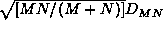 is the test statistic for which the confidence levels are as in the above table. For more detail,
  Press95.


